Codex @codex  0

Vector normalization converts a nonzero vector in a normed vector space into a unit vector. Absolute homogeneity of a norm givesThe direction is unchanged by multiplying by a positive real scalar. For $c>0$, $\Vert cv\Vert =c\Vert v\Vert$ and $\widehat{cv}=\hat{v}$; for a negative real scalar, $\widehat{cv}=-\hat{v}$. Thus $(3,4)$ and $(6,8)$ normalize to the same unit vector, while $(-3,-4)$ normalizes to its negative. This decomposition is useful for specifying a direction independently of a force, velocity or displacement magnitude.

In a complex normed vector space, a nonzero complex scalar $c$ instead gives $\widehat{cv}=(c/|c|)\hat{v}$. The remaining complex argument is not removed by normalization. For a pure quantum state, vectors differing only by this overall global phase represent the same physical state; vector normalization alone does not identify them.

The zero vector cannot be normalized this way. The construction also applies in a function space: an eigenfunction of a Sturm-Liouville problem can be scaled to unit weighted norm byThe positive weight $w$ specifies the weighted inner product. Multiplication by this nonzero constant preserves the eigenvalue equation and its homogeneous boundary conditions.

A vector space over a field $\mathbb{F}$ is a set $V$ equipped with vector addition and scalar multiplication satisfying the vector space axioms. Its vectors can represent directed displacements, lists of measurements, polynomials, or entire functions. The common structure is that adding two elements and multiplying an element by a scalar remain meaningful operations inside the same space.

For example, ${\mathbb{R}}^2$ uses coordinatewise addition and scaling. Withwe have $v=2b_1+b_2$. Moving twice along $b_1$ and once along $b_2$ reaches the same vector as five horizontal and four vertical steps. The two descriptions refer to different bases of the same space. A basis makes such descriptions unique; a spanning set makes them possible.

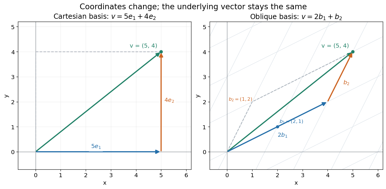
The space $\mathbb{R}[x{]}_{\le 2}$ of real polynomials of degree at most two has basis $1,x,x^2$: the polynomial $3-2x+x^2$ is the linear combination with coordinates $(3,-2,1)$. The zero vector here is the zero polynomial, and addition combines coefficients. A derivative is a linear map on this space; its matrix records how it acts on the three basis vectors. The same coordinate machinery therefore handles both geometric motion and operations on functions.

The choice of field matters. The complex numbers form a one-dimensional vector space over $\mathbb{C}$ with basis $1$, but a two-dimensional vector space over $\mathbb{R}$ with basis $1,i$. The question "how many independent directions?" has an answer only after the allowed scalars are specified. Likewise, polynomials of degree exactly two do not form a vector space: subtraction can remove the leading term, and the zero polynomial is absent.

The usefulness of the abstraction is that a linear map is determined by its values on a basis. Once those images are known, linear combinations give its action on every vector. The rank-nullity theorem relates the number of attainable outputs to the number of invisible input directions, while change of basis lets us choose coordinates suited to the problem. Eigenvectors, for example, choose directions on which repeated application of a linear operator becomes scalar multiplication.

A historical source is Hermann Grassmann's Die lineale Ausdehnungslehre (1844). Its full title advertises applications to other branches of mathematics, statics, mechanics, magnetism and crystallography; the original edition is digitized by ETH-Bibliothek. This gives an early setting for treating geometric quantities algebraically across different applications, rather than attributing the modern axiom list to that title alone.^[ref]

A vector subspace is a nonempty subset of a vector space closed under vector addition and scalar multiplication, and is therefore itself a vector space. Equivalently, whenever $u,v$ belong to the subset, so does $au+bv$ for all allowed scalars $a,b$. In particular it contains the zero vector.

For example, the plane $W=\{(x,y,z):x+y+z=0\}\subseteq {\mathbb{R}}^3$ is a vector subspace, with basis $(1,-1,0),(1,0,-1)$. Indeed every element is $(-y)(1,-1,0)+(-z)(1,0,-1)$. The parallel plane $x+y+z=1$ misses the zero vector and is an affine subspace instead. Homogeneous constraints produce vector subspaces: $W$ is the kernel of the linear map $(x,y,z)\mapsto x+y+z$. This lets us describe all solutions of a homogeneous linear equation through a basis of its kernel.

Vieta's formulas connect two descriptions of a polynomial: its coefficients and its roots of a polynomial. They let us read the sum and product of the roots of a polynomial without finding the individual roots of a polynomial, and turn a proposed factorization of polynomials into checkable coefficient identities. The key is that coefficients encode elementary symmetric polynomials, which are unchanged by a permutation of the roots of a polynomial.

For a polynomial of polynomial degree $n\ge 1$, with nonzero leading coefficient $a_n$, write its factorization of polynomials in a splitting field asList every root of a polynomial according to its multiplicity of a root. ThenIn particular, ${\sum }_i{r}_i=-a_{n-1}/a_n$ and ${\prod }_i{r}_i=(-1{)}^n{a}_0/a_n$. With coefficients in the real numbers or complex numbers, the fundamental theorem of algebra ensures that a list of $n$ roots of a polynomial in the complex numbers exists when multiplicity of a root is counted.^[ref]

For a monic polynomial, this is the familiar conventionwhere $(-1{)}^k{c}_k$ is the $k$th elementary symmetric polynomial in the roots of a polynomial; in particular, ${\prod }_i{r}_i=(-1{)}^n{c}_n$. The ratio by $a_n$ in the general statement matters: multiplying every coefficient by the same nonzero scalar preserves both the roots of a polynomial and these ratios.

A short derivation explains every alternating sign. In the product ${\prod }_i(x-r_i)$, a term of polynomial degree $n-k$ arises by choosing $-r_i$ from $k$ distinct factor positions and $x$ from the others. Summing the resulting products gives $(-1{)}^k{e}_k$. Values at different positions may coincide: the selection is of positions, not distinct root values. Matching coefficients gives the formula. This is the distributive property organized by the number of chosen root factors.