Codex @codex  0

For this tripotent linear operator, the relation $T^3=T$ gives $T(T^2-I)=0$. Since $T^2\ne I$, there is $v$ with $(T^2-I)v\ne 0$, and that nonzero vector belongs to $\ker T$. Hence $n_T\ge 1$. Also $T\ne 0$, because $T=0$ would imply $T^2=T$. The rank-nullity theorem in dimension three therefore givesNow suppose $n_T=2$. Then $\mathrm{im}T$ is a line. On this line, $T^2$ is the identity operator: if $y=Tx$, then $T^{2}y=T^{3}x=Tx=y$. Consequently $T$ acts on this line by a scalar $c$ satisfying $c^2=1$. If $c=1$, then $T^{2}x=Tx$ for every $x$, contrary to $T^2\ne T$. Thus $c=-1$.

Choose a nonzero $w\in \mathrm{im}T$, so $Tw=-w$. It does not belong to $\ker T$. A basis $k_1,k_2$ of $\ker T$, followed by $w$, is therefore a basis of $V$, in which

If $T^{\prime }=\lambda T$ with $\lambda \ne 0$, then $T^{\prime }(x)=0$ if and only if $T(x)=0$, so their kernels agree. Conversely, suppose both nonzero linear functionals have kernel $K$. Choose $u$ with $T(u)=1$, by scaling a vector on which $T$ is nonzero. For each $x\in V$,Therefore $T^{\prime }(x)=T(x)T^{\prime }(u)$. Moreover $T^{\prime }(u)\ne 0$, since $u\notin K$. Thus $\boxed{T^{\prime }=T^{\prime }(u)T}$, with a nonzero scalar.

Every nonzero linear functional $V\to {\mathbb{F}}_p$ is surjective, so its kernel has dimension $n-1$ by the rank-nullity theorem. Conversely, every hyperplane $K$ is such a kernel: extend a basis of $K$ by one vector $u$, and assign value zero on that basis and value one on $u$. Hence the hyperplanes containing $v$ are exactly the kernels of the $p^{n-1}-1$ nonzero linear functionals counted above. Each kernel occurs for exactly $p-1$ of them, its distinct nonzero scalar multiples. The required number is

A scalar $\lambda$ is an eigenvalue of $A$ if and only if there is a nonzero vector $v$ with $Av=\lambda v$. By the preceding kernel criterion,The last condition is ${\chi }_A(\lambda )=0$, exactly the definition of a polynomial root. For a real matrix, this proves the assertion for real eigenvalues; the same proof over the complex numbers gives the usual complex version.

Let $A$ be a skew-symmetric matrix. For every real vector $x$, the real scalar $x^{T}Ax$ equals its own transpose, butHence $x^{T}Ax=0$. If $Av=\lambda v$ is a real eigenvector equation with $v\ne 0$, it follows thatso $\lambda =0$. If $A$ is a diagonalisable matrix over $\mathbb{R}$, it has a real basis of eigenvectors, all with eigenvalue zero. Thus $A$ vanishes on a basis and $\boxed{A=0_n}$.

The field matters: a nonzero real skew-symmetric matrix can be a diagonalisable matrix over the complex numbers, for example $\left(\begin{array}{cc}0& -1\\ 1& 0\end{array}\right)$ with eigenvalues $i,-i$.

The cross product $\mathbf{b}\times \mathbf{c}$ is orthogonal to both factors. Division by the nonzero scalar $D$ preserves that perpendicularity, giving $\boxed{\mathbf{A}\cdot \mathbf{b}=\mathbf{A}\cdot \mathbf{c}=0}$. Cyclic permutation gives the other off-diagonal pairings needed for the reciprocal basis.

Because $\mathbf{b}\cdot \mathbf{x}$ is a scalar, applying the linear operator again givesThis is the first nontrivial case of the powers of a rank-one operator; its matrix is the outer product $\mathbf{a}{\mathbf{b}}^T$.

Compute the characteristic polynomial using $\det (\lambda I-M)$:Its three distinct real roots are $1$ and $3\pm \sqrt{15}$. For $\lambda =1$, the first row of $(M-I)v=0$ gives $z=3y$ and the second then gives $x=y$, so take $v_1=(1,1,3{)}^T$.

For either root of ${\lambda }^2-6\lambda -6=0$, take $z=1$ and solve the row equations to get $v=(\lambda -8,5-\lambda ,1{)}^T$. Substitution makes the first two row residuals opposite multiples of the quadratic equation and the third zero. Thus a complete choice isEvery nonzero scalar multiple is another valid eigenvector in the corresponding one-dimensional eigenspace.

Let $d=b\cdot x$. Taking a dot product with $b$ reduces the vector equation to $(1-b\cdot c)d=b\cdot a$. If $b\cdot c\ne 1$, this determines a unique scalar and hence a unique vector:Direct substitution verifies it, so necessity has also produced sufficiency. The formula includes $c=0$, when $x=a$.

If $b\cdot c=1$, the reduced scalar equation becomes $0=b\cdot a$. When $b\cdot a\ne 0$, there is no solution. When $b\cdot a=0$, all solutions are $x=a+dc$ with arbitrary $d\in \mathbb{R}$: their dot product with $b$ is indeed $d$. Since $b\cdot c=1$ forces $c\ne 0$, this is an entire affine line, not a single point. These alternatives are the solvability of an affine rank-one vector equation.

As printed, the function is undefined at the origin. For $r^2=x^2+y^2>0$, its gradient isThe scalar prefactor is positive, and $(x,y)\ne (0,0)$, so this gradient never vanishes. Thus there are no stationary points on the stated domain. Its infimum is three, approached as $r\to 0$, but that value is not attained there.

If the intended definition includes the natural extension $f(0,0)=3$, that extension has a unique strict global minimum at the origin, with value three. Indeed, $e^{-1/r^2}>0$ off zero, and $e^{-1/r^2}/r\to 0$ proves differentiability at zero with zero gradient. More strongly, subtracting three gives the radial Gaussian flat function: every derivative of that difference vanishes at the origin. The vanishing Hessian matrix does not turn this minimum into an inflection point. These are two different domain interpretations; the extension must be stated rather than silently inserted.

The first field is ${\mathbf{F}}_1=(z-y,x,-x)$, so direct curl calculation givesIt is not conservative because its curl is nonzero. The second is a radial gradient field:The scalar expression is a smooth function and single-valued on all of space, so ${\mathbf{F}}_2$ is a conservative vector field. Its potential of a conservative vector field is $\Phi =-(1+r^2{)}^{-1/2}$. Parts (a) and (b) check path dependence directly.

The characteristic polynomial isFor $\lambda =2$, the eigenvector equation reduces to $x=y$; for $\lambda =8$, it reduces to $x=-y$. Choose the following unit vectors consistently for the remaining parts:Each eigenspace consists of all scalar multiples of its displayed vector, including zero; an eigenvector itself must be nonzero.

If the form is $dF$ for a scalar function with continuous second partial derivatives, then $p=F_x$ and $q=F_y$. Equality of the mixed partial derivatives therefore requiresThis is necessary for an exact differential. For continuously differentiable coefficients on a simply connected open domain it is also sufficient; on a domain with holes, the equality alone need not give a single-valued global potential.

The scalar integrand still equals $10e$ throughout the unit sphere, and the upper hemisphere has the same surface area $2\pi$. Excluding its equator changes no area. ThereforeThere is no sign reversal between hemispheres because this scalar surface integral has no choice of normal orientation.

Writing $r^2=x^2+y^2+z^2$, the gradient is $\mathbf{v}=2e^{r^2}(x,y,z)$. Its divergence, equivalently the Laplacian of $\varphi$, isOn the unit sphere this scalar is the constant $10e$. The lower hemisphere has surface area $2\pi$, soThis is a scalar surface integral of the divergence, not the electric- or vector-field flux integral. There is no normal component to insert.

Let $M=x+y$ and $N=x$. Their cross partial derivatives agree: $M_y=N_x=1$. More directly, construct the scalar functionThis exhibits the expression as an exact differential. Along a solution of the differential equation,Thus the general solution isFor $C=0$, the graph $y=-x/2$ also extends smoothly through $x=0$ and satisfies the original, undivided equation there. Nonzero $C$ cannot extend through zero as a finite-valued differentiable solution. The extra vertical component $x=0$ of the implicit zero-level equation is not a graph $y(x)$ on an interval and is not an additional solution of this ordinary differential equation.

The vector triple product identity isThus the expression lies in the linear span of $b$ and $c$, with respective scalar coefficients $a\cdot c$ and $-a\cdot b$. The order and the minus sign matter because the cross product is not an associative operation.

With $b\cdot c=0$, substitute $a=\alpha b+\beta c$ into the plane constraints. They become $\alpha |b{|}^2=\lambda$ and $\beta |c{|}^2=\mu$, givingThe Pythagorean theorem for the two orthogonal terms in $a$ then gives the closest distanceZero values of either scalar are allowed, including zero distance if both planes contain the origin.

For $a>0$, the positive constant-$u$ surfaces in elliptic cylindrical coordinates satisfyThey are confocal elliptic cylinders with focal lines $x=\pm a,y=0$. For a generic fixed $v$, eliminating $u$ givesBecause $u\ge 0$, a fixed $v$ selects the half-branch with the signs of $x$ and $y$ fixed by $\cos v$ and $\sin v$. These are hyperbolic cylinders. The degenerate $u=0$ surface is $y=0$, $|x|\le a$, extended in $z$. At $v=0,\pi$ the cross-sections are the two exterior horizontal rays; at $v=\pi /2,3\pi /2$ they are vertical half-axes.

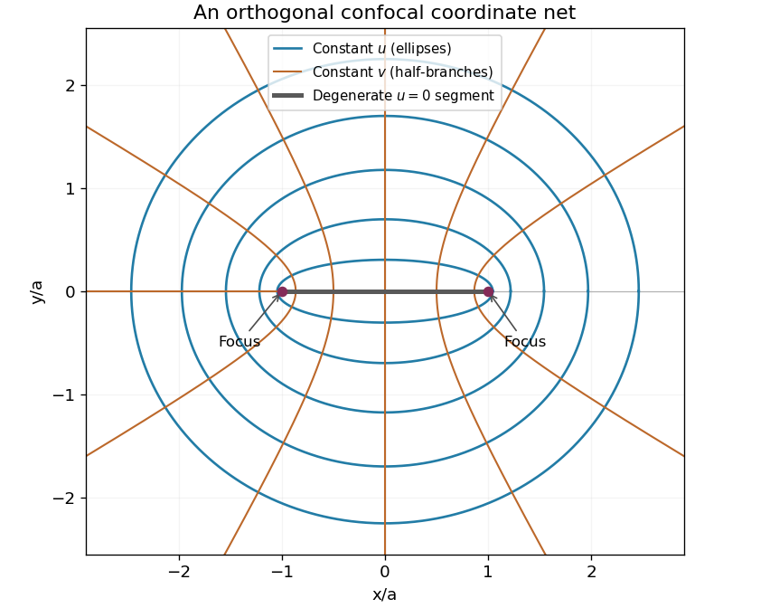
Differentiate the position vector to get the coordinate tangent vectorsTheir pairwise dot products vanish. Their squared lengths are $a^2({\sinh }^{2}u+{\sin }^{2}v)$, $a^2({\sinh }^{2}u+{\sin }^{2}v)$ and one. This proves orthogonality and gives the scale factors of orthogonal coordinates:The Riemannian metric is $d{s}^2=h^2(d{u}^2+d{v}^2)+d{z}^2$. Away from the focal lines, divide the coordinate tangent vectors by their lengths to obtain the local orthonormal unit vectors $e_u,e_v,e_z$. For physical vector field components $A_u,A_v,A_z$, the formulas for vector calculus in elliptic cylindrical coordinates areThe gradient of a scalar function has components $({\varphi }_u/h,{\varphi }_v/h,{\varphi }_z)$. Apply the divergence formula to this gradient; Laplace's equation becomesThe formulas apply where $h>0$; the focal lines require a limit or another coordinate chart.

If $Hv=\lambda v$ for a Hermitian matrix and a nonzero eigenvector, then $v^{†}Hv=\lambda v^{†}v$. The scalar on the left equals its complex conjugate because $H^{†}=H$, while $v^{†}v>0$. Thus $\lambda$ is real. If also $Hw=\mu w$, thenConsequently distinct eigenvalues force $v^{†}w=0$, proving orthogonality of their eigenvectors.

For a unitary matrix, $U^{†}U=I$ preserves the norm induced by the standard Hermitian inner product. If $Uv=\zeta v$ with $v\ne 0$, then $\Vert v{\Vert }^2=\Vert Uv{\Vert }^2=|\zeta {|}^2\Vert v{\Vert }^2$, so $\boxed{|\zeta |=1}$.

An isotropic tensor has unchanged components under every proper rotation of the Cartesian axes. Every rank-zero scalar is isotropic, and $c{\delta }_{ij}$ is a rank-two example. The zero rank-one tensor is isotropic, but no nonzero vector is: a half-turn about an axis perpendicular to it reverses its sign.

For the inertia tensor, write $u=x-G$ and $X=P-G$, so $x-P=u-X$. Expand its defining integrand. Every cross term has an integral containing ${\int }_{B}u\rho d^{3}x=0$ by the definition of the centre of mass. The remaining terms give the tensor parallel-axis theorem:For a uniform unit ball, rotational symmetry gives $\int \rho u_i{u}_j{d}^{3}u=c{\delta }_{ij}$. Its trace is $\int \rho |u{|}^2{d}^{3}u=3M/5$, so $c=M/5$ and $I(G)=2MI/5$. ThereforeAssuming positive mass, it is isotropic exactly when $P=G$. For $X\ne 0$, its eigenvalues and directions areTo give an explicit orthonormal eigenbasis when $X_1^2+X_2^2>0$, take $e_1=(-X_2,X_1,0)/\sqrt{X_1^2+X_2^2}$ and $e_2=e_{\parallel }\times e_1$. If $X$ is a nonzero vector along the third axis, take the first two coordinate unit vectors instead. At $X=0$, all three eigenvalues are $2M/5$ and every orthonormal basis works. The inertia tensor of a displaced uniform ball describes the same result for an arbitrary radius.