Codex @codex  0

A finite-dimensional density operator $\rho$ represents a quantum state on a Hilbert space. It is Hermitian, positive semidefinite, and has trace one:The density matrix is its matrix in a chosen orthonormal basis. In dimension $N$ it has $N^2-1$ real parameters: a Hermitian matrix has $N^2$, and fixing its trace removes one; positivity restricts the allowed values.

A quantum state ensemble of normalized pure states $|{\psi }_i⟩$ with positive probabilities $p_i$ givesZero-weight terms can be omitted. Conversely, the spectral theorem gives such an ensemble for every density operator, using its orthonormal eigenvectors and nonnegative eigenvalues, with zero eigenvalues omitted. A pure state has $\rho =|\psi ⟩⟨\psi |$; a mixed state needs at least two nonzero eigenvalues. ^[ref]

For a projective measurement with orthogonal projections ${\Pi }_a$, the Born rule isThis is the average of the component pure state probabilities. Positivity makes each outcome probability nonnegative, and ${\sum }_a{\Pi }_a=I$ makes them sum to one. The same density operator therefore predicts every measurement on the system without requiring a unique preparation history. ^[ref]

For a closed system, Schrödinger picture evolution under a unitary operator iswhen ${\rho }_H={\rho }_S(0)$ denotes the time-independent Heisenberg picture state and $U(0)=I$. In the Schrödinger picture the density operator evolves; in the Heisenberg picture the observables evolve instead, with identical measurement predictions. This unitary operator preserves the eigenvalues and hence the purity of a density operator. ^[ref]

A historical source for the probabilistic formulation of quantum mechanics is von Neumann's 1927 paper Wahrscheinlichkeitstheoretischer Aufbau der Quantenmechanik. ^[ref]

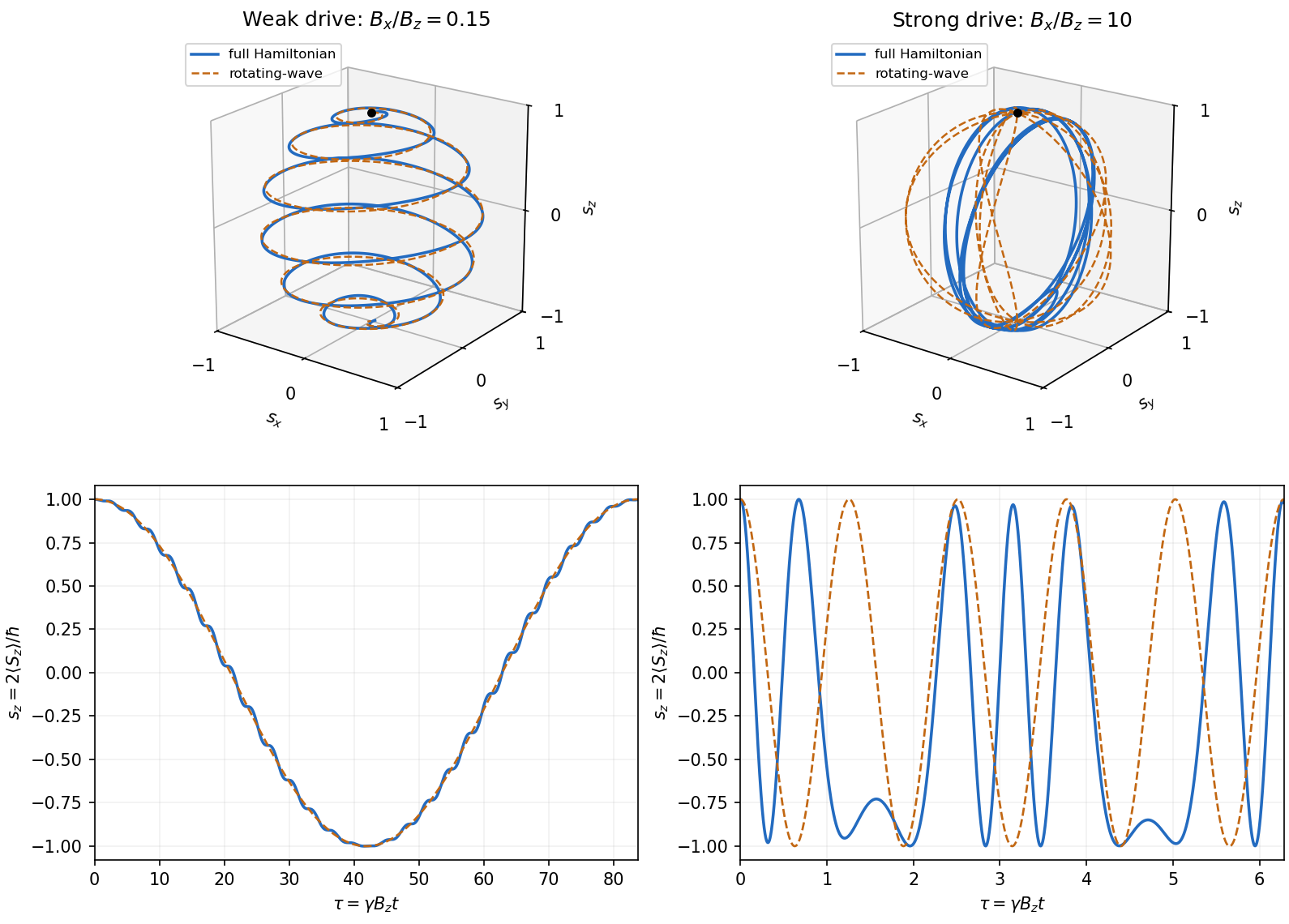
For $H=-\gamma B_z{S}_z-\gamma B_x{S}_x\cos (\omega t)$, choose ${\omega }_z=\gamma B_z>0$ and nominal resonance $\omega ={\omega }_z$. Starting from up spin, the rotating-wave approximation gives the normalized Bloch vector in the title, with signed $\Omega =\gamma B_x/2$. It follows by transforming the spinor $(\cos (\Omega t/2),i\sin (\Omega t/2){)}^T$ from the interaction picture back to the Schrödinger picture. Thus weak transverse driving combines slow meridional Rabi oscillations with fast Larmor precession.

This result requires $|B_x|\ll |B_z|$ and cannot be extrapolated as a controlled strong-drive formula. The exact equation is $\dot{\mathbf{s}}=\gamma \mathbf{s}\times (B_x\cos \omega t,0,B_z)$. For $|\gamma B_z|t\ll 1$, neglecting the bias gives the controlled leading solutionThe fixed-axis driving generators commute at all times, making this solution exact when the bias is zero at any prescribed drive frequency. At nominal resonance in a strong-drive experiment, the initial rotation scale is $\Theta \simeq \gamma B_{x}t$, twice the incorrectly extrapolated rotating-wave rate. Bias effects must be retained on longer times.

At resonance, retain the signed coupling $\Omega =\gamma B_x/2$. In the interaction picture, the given solution reduces to $c_1=\cos (\Omega t/2)$ and $c_2=i\sin (\Omega t/2)$. Returning to the Schrödinger picture givesFor a normalized spinor $(a,b{)}^T$, the Pauli matrices give $⟨\mathbf{\sigma }⟩=(2\mathrm{Re}{a}^{\ast }b,2\mathrm{Im}{a}^{\ast }b,|a{|}^2-|b{|}^2)$. Therefore the spin expectation value within the rotating-wave approximation isIts magnitude is $\hslash /2$: the Bloch vector stays on the unit sphere. In a frame rotating about $z$ at angular velocity $-{\omega }_z$, it makes a uniform rotation in the $yz$ plane. For $|B_x|\ll |B_z|$, this gives slow Rabi oscillations between the poles, accompanied by rapid laboratory Larmor precession about $z$.

If the same formula is formally used for $|B_z|\ll |B_x|$, it predicts fast meridional rotations whose plane turns slowly about $z$. However, the original PDF really does ask for this opposite limit, and it lies outside the assumption used in part (b). That formal description is not a controlled prediction for the stated linearly driven Hamiltonian operator.

A valid strong-drive description starts from the exact equation for the Bloch vector $\mathbf{s}=2⟨\mathbf{S}⟩/\hslash$:For times $|\gamma B_z|t\ll 1$, neglecting the weak bias gives a controlled leading approximation, since the time integral of the omitted Hamiltonian operator has small norm. The remaining field has a fixed $x$ axis, so its generators commute at different times andAt the nominal resonance $\omega =\gamma B_z$ and on the early spin-rotation scale $t\sim 1/|\gamma B_x|$, this becomes $\Theta \simeq \gamma B_{x}t$. The initial rotation rate is consequently $\gamma B_x$, twice the rate predicted by extrapolating the rotating-wave approximation. For longer times the exact differential equation must be retained. The following original calculation illustrates both regimes rather than asserting an exact strong-drive Rabi formula.

For the requested oscillator response, treat $y$ as the fixed transverse position of a one-dimensional quantum harmonic oscillator along $z$, and put $\theta =ky$. The supplied radiation is transverse and already satisfies the Coulomb gauge. Its perturbation isThe annihilation operator and creation operator giveThus the only first-order transition out of the ground state is to $|1⟩$. More generally, the oscillator electric-dipole selection rule is $\Delta n=\pm 1$. This is a rule for matrix elements; exact energy conservation is replaced by a finite-time resonance profile during a switched finite-duration interaction.

To display both the resonant and nonresonant terms without spurious singularities, defineThe interaction picture coefficient in the given expansion is thenThe full Schrödinger picture coefficient of $|1⟩$ is $e^{-3i{\omega }_{0}t/2}{b}_1(t)$, while that of $|0⟩$ is $e^{-i{\omega }_{0}t/2}$ at this order. The normalization changes only at order $A_0^2$. In particular, at $\omega ={\omega }_0$ the first term is $C{e}^{i\theta }t$, finite for every finite time, and the perturbative result requires $|b_1|\ll 1$.

The fixed-$y$ interpretation is needed for the displayed target formulae. If $p^2$ were instead a three-dimensional kinetic operator with no transverse confinement, that model would have no normalizable transverse ground state, and $e^{\pm iky}$ would transfer transverse momentum $\pm \hslash k$. A treatment of that different model needs specified transverse states and recoil energies; they are absent from the question. The following parts use the intended localized-oscillator response.

For the complex scalar field, the canonical momenta are $\pi ={\dot{\varphi }}^{†}$ and ${\pi }^{†}=\dot{\varphi }$. Split $H=H_0+H_I$. The interaction picture is obtained from the Schrödinger picture by $|{\Psi }_I(t)⟩=e^{i{H}_{0}t}|{\Psi }_S(t)⟩$ and $O_I(t)=e^{i{H}_{0}t}{O}_S{e}^{-i{H}_{0}t}$, choosing a common time origin. The fields therefore obey the free Klein-Gordon equation, while the states evolve through $H_I(t)$. The canonical quantization of a complex scalar field givesThe adjoint expansion contains $a^{†}$ and $b$. Particle and antiparticle modes are independent; their nonzero commutators areAll cross-species commutators, and all pairs of creation operators or of annihilation operators, vanish. These formulas reproduce $[\varphi (\mathbf{x}),\pi (\mathbf{y})]=[{\varphi }^{†}(\mathbf{x}),{\pi }^{†}(\mathbf{y})]=i{\delta }^{(3)}(\mathbf{x}-\mathbf{y})$ and the remaining vanishing equal-time commutators.

There are no derivative interactions, so the interaction Hamiltonian is $H_I(t)=-\int d^{3}x{\mathcal{L}}_I(x)$. Differentiating the interaction picture state gives $i{\partial }_t|{\Psi }_I⟩=H_I(t)|{\Psi }_I⟩$. Its time-evolution operator satisfiesIteration gives ordered integration regions $t_1>\cdots >t_n$. Each is $1/n!$ of the full region with a time-ordered product, yielding the Dyson seriesWith the usual asymptotic scattering prescription, taking $t_0\to -\infty$ and $t\to +\infty$ provesTime ordering is essential because different interaction Hamiltonians need not commute.

At first order, use the connected tree scattering amplitude, equivalently the normal-ordered quartic vertex with the vacuum and one-particle mass contributions removed. This qualification matters if the local product is interpreted literally without normal ordering: single-vertex tadpole diagrams and vacuum diagrams are not the requested connected two-particle amplitude. The complex scalar quartic contact vertex is obtained fromIn a fully connected matrix element, an incoming particle and outgoing antiparticle attach to the two $\varphi$ factors; an outgoing particle and incoming antiparticle attach to the two ${\varphi }^{†}$ factors. Each pair has two assignments, giving $2!2!=4$. The external relativistic normalization of a one-particle state cancels each mode measure: for example $[\varphi (x),a^{†}(p_1)]=e^{-i{p}_{1}x}$ and $[b(q_2),\varphi (x)]=e^{i{q}_{2}x}$. Consequently the connected integrand is $4e^{-i(p_1+q_1-p_2-q_2)\cdot x}$, andThus the invariant connected amplitude isThe Dirac delta function expresses four-momentum conservation.

For the identity contribution, commute $a(p_2)$ through $a^{†}(p_1)$ and independently $b(q_2)$ through $b^{†}(q_1)$; all terms leaving a creation operator against the left Fock vacuum or an annihilation operator against the right Fock vacuum vanish. HenceThere is no exchange term between the two distinct particle and antiparticle species.

For a time-independent Hamiltonian operator and a Schrödinger picture observable with no explicit time dependence, the Heisenberg picture operator isDifferentiation gives ${\dot{O}}_H=iH{O}_H-i{O}_{H}H=i[H,O_H]$, soIf $O_S$ itself depends explicitly on time, one must add $e^{iHt}({\partial }_t{O}_S)e^{-iHt}$ to ${\dot{O}}_H$; the displayed commutator relation uses the usual convention of no explicit time dependence for the observable.

In the Schrödinger picture, a time-independent Hamiltonian gives $|{\psi }_S(t)⟩=U(t)|\psi (0)⟩$, where $U=e^{-iHt/\hslash }$. The Heisenberg picture transfers this evolution to each observable:Both pictures give the same probabilities and expectation values. Differentiating yields the Heisenberg equation of motionThe last term is an explicit change of the measured operator. If it is absent and $[H,A]=0$, the observable is conserved.

The corresponding classical equation is $dA/dt=\{A,H{\}}_{\mathrm{PB}}+\partial A/\partial t$. The correspondence principle relates the Poisson bracket to $[A,H]/(i\hslash )$, with suitable operator ordering and a classical limit. For $H=p^2/(2m)+V(x)$, the canonical commutation relation givesTaking means gives Ehrenfest theorem. Its second equation contains $-⟨V^{\prime }(x)⟩$, which need not equal $-V^{\prime }(⟨x⟩)$. A narrow wave packet in a slowly varying force field can follow the classical equations approximately; a quadratic potential makes the equality exact for the means.

For a quantum harmonic oscillator, direct solution gives $x_H(t)=x_H(0)\cos \omega t+p_H(0)\sin \omega t/(m\omega )$ and $p_H(t)=p_H(0)\cos \omega t-m\omega x_H(0)\sin \omega t$. These have the classical form as operator identities. A coherent state supplies a localized center moving on the classical orbit, whereas an energy eigenstate has stationary density and $⟨x⟩=0$, even at large excitation. Thus large quantum numbers alone do not create a localized classical trajectory. Classical behavior also concerns state preparation, relative fluctuations and the resolution of the measurements.

Time dependence in quantum mechanics describes how a prepared quantum state changes and thereby changes the probabilities of later measurements. For an isolated system, the Schrödinger picture assigns this evolution to a state vector $|\psi (t)⟩$, governed by the Time-dependent Schrödinger equationThe Hamiltonian is a self-adjoint operator; it has units of energy, while $\hslash$ has units of action, so $\hat{H}/\hslash$ has units of inverse time. For a particle with potential energy $V(\mathbf{r},t)$, this becomesGiven a suitable initial wavefunction and the physical boundary conditions, this first-order equation determines its subsequent propagation. Its linearity means that the evolution of a quantum superposition is the corresponding quantum superposition of evolved states.

For a real potential energy, this equation and its complex conjugate imply the local continuity equationHere $\rho$ is the probability density and $\mathbf{j}$ the probability current. Vanishing net boundary flux preserves wavefunction normalization, as required by the Born rule.

The time-evolution operator packages the solution for every initial state:Because ${\hat{H}}^{†}=\hat{H}$, differentiation givesTherefore $U^{†}U=I$: this is unitary time evolution, preserving inner products and all state norms. It is reversible, with $U(t,t_0{)}^{-1}=U(t_0,t)=U(t,t_0{)}^{†}$, and obeys the composition law $U(t_2,t_0)=U(t_2,t_1)U(t_1,t_0)$.

For a time-independent Hamiltonian, the solution is the operator exponentialIf the Hamiltonian varies with time, the analogous simple exponential of its integral is valid when $[\hat{H}(t),\hat{H}(t^{\prime })]=0$ for all relevant times. Otherwise time ordering is essential:The meaning is explicit in the first terms of the ordered series,the later-time operator stands on the left. In the position representation, the same propagation is expressed by the quantum-mechanical propagatorIts initial value is the Dirac delta function ${\delta }^3(\mathbf{r}-{\mathbf{r}}^{\prime })$.

A time-independent Hamiltonian has energy eigenstates satisfying $\hat{H}|n⟩=E_n|n⟩$. A single such initial state evolves asIt is a stationary state: its global phase changes, but its probability density and the distributions of time-independent observables do not. Its energy is sharp. Any quantum superposition entirely within one degenerate energy eigenspace also acquires one common global phase and is stationary. Stationarity does not require zero probability current; for instance, $u_n(\varphi )=e^{in\varphi }/\sqrt{2\pi }$ on the ring has a constant density and persistent circulation when $n\ne 0$.

An arbitrary normalized state can instead contain different energy eigenvalues:A continuous spectrum requires corresponding integrals. For the discrete case, an energy measurement gives $E_n$ with fixed probability $|c_n{|}^2$ (summed over degeneracies), but relative quantum phases change with time. ConsequentlyThe interference terms can oscillate at angular frequencies $(E_m-E_n)/\hslash$. For two populated energy levels, this supplies a characteristic period $2\pi \hslash /|E_m-E_n|$ when the interference term is nonzero. Thus fixed energy populations do not imply a stationary spatial distribution.

For a normalized state and an observable $\hat{A}(t)$, its expectation value isThis is the statistical mean over repeated preparations and measurements. In an eigenbasis of energy eigenstates for a time-independent Hamiltonian and a time-independent $\hat{A}$,Only matrix elements connecting different energies can generate these oscillations. If $[\hat{A},\hat{H}]=0$, its expectation value is constant for every initial state, provided it has no explicit time dependence.

Differentiating the expectation value and substituting the Schrödinger equation for both the bra and ket proves the general Ehrenfest theorem:Equivalently,These manipulations require the state to lie in the relevant operator domains. Taking $\hat{A}=\hat{H}$ gives $d⟨H⟩/dt=⟨{\partial }_t\hat{H}⟩$, so energy is conserved under a time-independent Hamiltonian.

For $\hat{H}={\hat{p}}^2/(2m)+V(\hat{x})$, the canonical commutation relation givesHence the particularly useful position-and-momentum form of Ehrenfest theorem isIt resembles Newton's second law, but the mean force generally differs from the force at the mean position. If a narrow wave packet samples a region where the force varies little, $⟨V^{\prime }(x)⟩\simeq V^{\prime }(⟨x⟩)$ gives approximate classical motion. For a quadratic potential energy this replacement is exact. In particular the quantum harmonic oscillator obeysThe centroid follows the classical harmonic oscillator, although this does not specify the full evolving wavefunction or its width.

The Heisenberg picture expresses the same physics by assigning evolution to observables instead:The expectation value is unchanged, and differentiation yields $d{\hat{A}}_H/dt=(i/\hslash )[{\hat{H}}_H,{\hat{A}}_H]+U^{†}({\partial }_t{\hat{A}}_S)U$. Thus state propagation, evolving expectation values, and the classical correspondence in Ehrenfest theorem are mutually consistent descriptions of the same unitary time evolution.

The annihilation operator associated with the new coordinate $X=x-x_0$ isAs the initial state is the old vacuum,Equivalently, applying $a^{\prime }$ to the number-state expansion in part (c) and shifting its summation index returns $-\lambda$ times the same state. It is therefore a coherent state of the displaced oscillator.

The new Hamiltonian is $H=U_{\min }+\hslash \omega (a^{\prime †}{a}^{\prime }+1/2)$. In the Schrödinger picture its evolution givesConsequentlyThe displayed prefactor is only a global phase. Equivalently, in the Heisenberg picture $a^{\prime }(t)=a^{\prime }(0)e^{-i\omega t}$. The mean occupation $|\alpha (t){|}^2={\lambda }^2$ is constant, and $\hslash \omega ({\lambda }^2+1/2)$ reproduces the energy above the new minimum found in part (b). Its mean position and momentum likewise reproduce that part's oscillating wavepacket centre.