Separating power imbalance from mode mismatch in optical beating ($|\gamma |=I_{\mathrm{beat},\mathrm{pk}}/(2\sqrt{I_s{I}_{\mathrm{LO}}})$)

Separating power imbalance from mode mismatch in optical beating requires more information than a single modulation-depth reading. In the optical heterodyne modulation depth model, two effects multiply:The power ratio controls one term, while $\gamma$ describes the mode-overlap factor in optical heterodyne detection. A low beat depth can result from either effect or both.

Measure each arm separately with the same detector and collection geometry, subtracting dark current. For sufficiently close optical frequencies with the same detector responsivity, let the separate currents be $I_s$ and $I_{\mathrm{LO}}$. After correcting the receiver's beat-frequency response,This consistency bound for separately measured heterodyne arm powers requires $I_{\mathrm{beat},\mathrm{pk}}\le 2\sqrt{I_s{I}_{\mathrm{LO}}}$. An apparent value above unity indicates inconsistent calibration, background treatment, conditions or model assumptions.

For an original example, separate currents are $0.40$ and $0.10\mathrm{mA}$. Their power-imbalance limit is $m_{\max }=0.80$. A corrected beat depth $m=0.56$ means peak beat current $0.28\mathrm{mA}$ and overlap $|\gamma |=0.70$. If the electrical chain instead attenuates the beat amplitude by $0.75$ relative to DC and that effect is ignored, the apparent depth becomes $0.42$ and inferred overlap $0.525$.

NIST's physical receiver experiment matched the two optical modes and received photocurrent contributions; it separately corrected electrical loss and impedance mismatch when inferring receiver response and modulation.^[ref] Holding alignment fixed while changing one arm's power tests whether the corrected overlap remains constant. Source drift, changed polarization or aperture clipping during the separate-arm measurements can spoil that inference.

The consistency bound for separately measured heterodyne arm powers is the requirement that the corrected peak beat current not exceed the maximum permitted by the two separately measured arm currents:Here $I_1,I_2$ are positive, dark-corrected currents and $B$ is the beat amplitude after correcting the electrical frequency response. The same collection geometry, detector responsivity and stable illumination must apply to all three measurements, as in separating power imbalance from mode mismatch in optical beating.

The Cauchy-Schwarz inequality gives a short physical proof. Write the collected optical fields as vectors $u,v$ in the detector-weighted inner product, with squared norms proportional to $I_1,I_2$. Their cross term $J$ obeys $|J{|}^2\le I_1{I}_2$ and the beat amplitude is $B=2|J|$. Equivalently, their Gram matrixis a positive semidefinite matrix, so its determinant cannot be negative. This is an overlap constraint rather than an empirical correction factor.

Measurement uncertainty matters when interpreting an apparent violation. In an original example, $I_1=I_2=0.100\mathrm{mA}$ and $B=0.204\mathrm{mA}$ give $\hat{\gamma }=B/(2\sqrt{I_1{I}_2})=1.02$. Suppose the three readings have independent $1\%$ relative standard uncertainty. From $\delta \log \gamma =\delta \log B-(\delta \log I_1+\delta \log I_2)/2$, the relative uncertainty is approximately $\sqrt{1+1/4+1/4}\%=1.225\%$, giving $u(\hat{\gamma })\approx 0.0125$. The excess above unity is only about $1.6$ standard uncertainties; it does not establish a physical overlap above one. Correlated calibration influences change the variance of a corrected heterodyne overlap estimate.^[ref]

NIST's receiver experiment separately addressed optical mode/polarization matching, electrical losses and impedance mismatch.^[ref] Interleaving the two arm-current measurements with the beat measurement helps detect source drift. Dark subtraction, detector nonlinearity or a changed collection aperture can also produce inconsistent inputs to the bound.

The variance of a corrected heterodyne overlap estimate quantifies uncertainty in $\hat{\gamma }=B/(2\sqrt{I_1{I}_2})$, where $B$ is corrected peak beat current and $I_1,I_2$ are separately measured arm currents. The consistency bound for separately measured heterodyne arm powers requires the physical overlap not to exceed one, but measured estimates fluctuate.

For small errors, let $\mathbf{e}=(\delta B/B,\delta I_1/I_1,\delta I_2/I_2{)}^T$ have covariance $R$, and put $\mathbf{v}=(1,-1/2,-1/2{)}^T$. Linearization givesThus common influences can cancel rather than contribute three independent uncertainty terms. This is the covariance form of the primary measurement-propagation rule.^[ref]

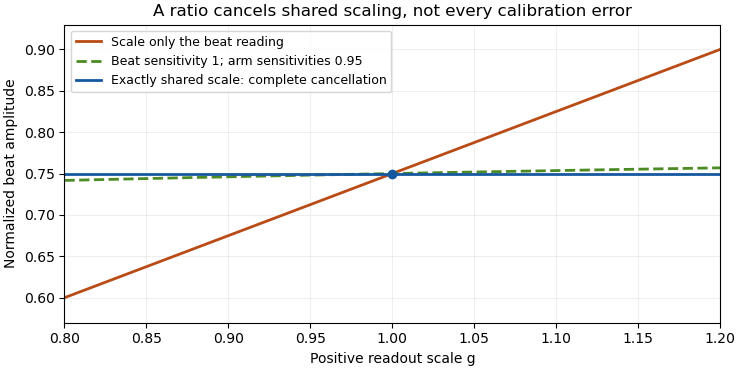
For an original model, all three current readings share a $2\%$ multiplicative calibration error, with additional independent $0.5\%$ errors on each. The common contribution to ${\mathbf{v}}^T\mathbf{e}$ is zero. The relative standard uncertainty is only $\sqrt{3/2}\times 0.5\%\approx 0.6124\%$, or $0.00490$ at overlap $0.80$. Treating the common calibration error as independent in all three readings would instead give about $2.525\%$ relative uncertainty.

The common-gain cancellation in heterodyne overlap uncertainty is exact for a single positive gain $g$: replacing $(B,I_1,I_2)$ by $(gB,g{I}_1,g{I}_2)$ leaves the ratio unchanged. A separate radio-frequency gain uncertainty affecting only $B$ does not cancel, nor does an additive dark-current offset generally have this property.

NIST's heterodyne receiver procedure corrected electrical loss and impedance effects separately from matching optical powers and modes.^[ref] Build the covariance from those actual shared and separate calibration paths. This first-order variance model also needs reconsideration when an arm current is close to zero or background subtraction makes its uncertainty comparable to its value.

Common-gain cancellation in heterodyne overlap uncertainty is the exact invariance of the normalized beat amplitudewhen the corrected peak beat current $B$ and both separately measured arm currents $I_1,I_2$ are multiplied by the same factor $g>0$. The factor occurs once in the numerator and once in the denominator. This is scale invariance: the ratio is a homogeneous function of degree zero. The cancellation holds for every realization of a random common factor, without requiring it to be independent of the currents.

More generally, take $B,I_1,I_2>0$ and let their residual multiplicative measurement calibration factors be $g_B,g_1,g_2$. The observed normalization satisfiesThus the gain-matching condition for heterodyne normalization is $g_B^2=g_1{g}_2$; the three factors need not all be equal. For example, $g_B=1$, $g_1=1.04$ and $g_2=1/1.04$ leave the ratio unchanged. The denominator depends on the geometric mean of its two factors.

Writing the natural logarithms of the factors as a random vector $\mathbf{G}$ makes the remaining uncertainty particularly clear. With $\mathbf{v}=(1,-1/2,-1/2{)}^T$,This identity is exact for the logarithmic error. The relative variance of the original ratio is only approximately equal to it when the errors are small, as in the variance of a corrected heterodyne overlap estimate. Keeping the covariance terms follows the general measurement-propagation rule.^[ref]

For an original imperfect-sharing model, set $\log g_j={\alpha }_{j}Z+{ϵ}_j$. Assume $Z,{ϵ}_B,{ϵ}_1,{ϵ}_2$ are zero-mean independent random variables. The coefficient of the shared fluctuation is $c={\alpha }_B-({\alpha }_1+{\alpha }_2)/2$, soTake ${\alpha }_B=1$, ${\alpha }_1={\alpha }_2=0.95$, with standard deviations $0.03$ for $Z$, $0.01$ for ${ϵ}_B$ and $0.004$ for each arm's separate error. Then $c=0.05$ and $v_d=0.00011025$, giving logarithmic standard uncertainty $0.0105$, approximately $1.05\%$ relative uncertainty. A large shared fluctuation can leave a small residual, but incomplete matching prevents exact cancellation.

If the log-errors additionally have a normal distribution, then $d\sim N(0,v_d)$ and the normalized readout has a lognormal distribution. Its exact expected value is $\gamma e^{v_d/2}$, not $\gamma$. At $\gamma =0.75$, this example gives mean $0.7500413$ and standard deviation $0.0078757$. The lognormal bias of a heterodyne overlap estimate comes from exponentiating the remaining error; the perfectly shared factor still cancels.

The physical calibration paths determine which model applies. NIST's receiver experiment combined two lasers through a beam splitter, polarizer and single-mode optical fiber, while separately correcting electrical loss and impedance mismatch.^[ref] An electronic gain change confined to the beat-frequency path need not appear in the arm-current measurements. Likewise, adding a current offset is not multiplication by a common factor. Background correction and the sharing of calibration factors must therefore be established before claiming cancellation.

Lognormal bias of a heterodyne overlap estimate is the upward mean shift that remains when a zero-mean Gaussian logarithmic error is exponentiated. It does not undo common-gain cancellation in heterodyne overlap uncertainty: a perfectly shared gain cancels in every reading, while residual mismatched gains can still fluctuate.

Write the normalized positive estimate as $\hat{\gamma }=\gamma e^d$, with fixed true overlap magnitude $\gamma$ and $d\sim N({\mu }_d,v_d)$. The moment-generating function of the normal distribution givesThese are exact lognormal distribution identities under the stated error model. When ${\mu }_d=0$, the logarithmic estimate is centered correctly and the median is $\gamma$, but the arithmetic mean exceeds it by relative amount $e^{v_d/2}-1$.

For an original deliberately visible example, $\gamma =0.8$ and logarithmic standard deviation 0.2 give $v_d=0.04$ and mean about 0.81616: a 2.02% mean shift. The values are chosen statistical parameters, not uncertainties reported for a receiver. An estimate can also exceed the physical consistency bound for separately measured heterodyne arm powers; the noisy readout is not itself a physical overlap above one.

If ${\mu }_d$ and $v_d$ are known, multiplying the estimate by $e^{-{\mu }_d-v_d/2}$ corrects its mean in this model. Uncertain variance in heterodyne lognormal bias correction matters when those parameters are estimated: plugging in a noisy variance, especially from related data, is not automatically an exact correction.

Averaging logarithms has a different interpretation from averaging overlaps. For $n$ independent zero-mean log-errors of variance $v_d$, the geometric mean is $\gamma e^{\overline{d}}$, whose arithmetic expectation is $\gamma e^{v_d/(2n)}$. A gain component shared across the entire run does not acquire the independent-shot $1/n$ variance reduction.

The physical calibration paths determine the logarithmic covariance. NIST's heterodyne apparatus controlled the optical modes while separately correcting electrical loss and impedance mismatch.^[ref] A first-order uncertainty calculation alone is not this exact distributional model; nonlinear effects and correlated inputs must be assessed explicitly.^[ref] State the assumed distribution and the intended summary rather than treating median, geometric mean and arithmetic mean as interchangeable.

Uncertain variance in heterodyne lognormal bias correction matters when a measured overlap is corrected using an estimated, rather than known, logarithmic variance. The known-variance correction is a nonlinear function of that estimate, so replacing the variance by an unbiased estimate does not automatically preserve unbiasedness of the corrected overlap.

Suppose $\hat{\gamma }=\gamma e^d$, with $d\sim N(0,v)$, and use $\tilde{\gamma }=\hat{\gamma }{e}^{-\hat{v}/2}$. If the variance estimate is independent of the overlap readout,Even if $\mathbb{E}[\hat{v}]=v$, Jensen's inequality gives $\mathbb{E}[e^{-\hat{v}/2}]\ge e^{-v/2}$. Consequently the mean corrected estimate is at least $\gamma$ under these independence and unbiased-variance assumptions. Equality requires a nonrandom variance estimate in the ordinary finite-variance case.

An original exact example uses a variance estimate from an independent normal calibration sample, with $\nu \hat{v}/v$ following a chi-squared distribution with $\nu$ degrees of freedom. Its Laplace transform givesThe logarithm of this factor is $v/2-(\nu /2)\log (1+v/\nu )$, which is positive for $v>0$. With stipulated $v=1$ and $\nu =2$, the factor is $e^{1/2}/1.5\approx 1.09915$: about a 9.91% remaining mean shift. This intentionally broad statistical example is not a typical receiver specification.

For fixed $v$ and large $\nu$, the logarithm is $v^2/(4\nu )+O({\nu }^{-2})$. More independent calibration information reduces this effect. Merely taking more overlap readings while retaining the same uncertain variance estimate does not remove its influence.

Dependent variance correction in heterodyne normalization requires the joint quantity $\mathbb{E}[e^{d-\hat{v}/2}]$ instead of the product of expectations above. A variance inferred from the same readout cannot simply be declared independent. Propagate the joint calibration and readout model, with a stated target summary. JCGM 101 treats input distributions from prior uncertainty calculations and numerical propagation explicitly.^[ref]

The optical gain-matching condition for heterodyne normalization still concerns physical calibration paths. This calculation addresses the statistical correction of residual log-errors; it does not imply that an imperfect RF or DC calibration can be repaired solely by subtracting a fitted variance.

Dependent variance correction in heterodyne normalization occurs when an overlap reading and the estimated logarithmic variance used to correct it share random information. Correcting the reading is then a joint nonlinear calculation; multiplying separately averaged correction factors can give the wrong answer, even when the variance estimate is unbiased.

Write $\hat{\gamma }=\gamma e^d$ and $\tilde{\gamma }=\hat{\gamma }{e}^{-\hat{v}/2}$, with $d$ a centered normal random variable of variance $v$. The exact mean ratio isThe joint exponential moment in overlap correction cannot generally be replaced by $\mathbb{E}[e^d]\mathbb{E}[e^{-\hat{v}/2}]$. That factorization requires independence. JCGM 101 treats a measurement function of jointly distributed inputs and distinguishes choosing that joint model from propagating it.^[ref]

An original counterexample takes $\hat{v}=d^2$. This estimate is nonnegative and has expected value $v$, because the log-error mean is assumed known to be zero. It is completely dependent on the reading. It is a mathematical stress test, not a recommended way to estimate receiver noise from one observation.

Completing the square in a Gaussian integral givesSetting $a=t=1$ therefore yieldsAt stipulated $v=1$, the ratio is $e^{1/4}/\sqrt{2}\approx 0.90794$. An unbiased variance estimate has left a downward mean shift. The independence-based upward-shift argument in uncertain variance in heterodyne lognormal bias correction does not apply.

For comparison, let $d^{\prime }$ be an independent copy and use $\hat{v}=(d^{\prime }{)}^2$. The variance estimate has exactly the same marginal distribution, but the mean ratio becomes $e^{v/2}/\sqrt{1+v}$, approximately 1.16582 at $v=1$. Changing only the dependence reverses the direction of the residual bias. Both are illustrative probability models, not measured optical noise levels.

In a physical analysis, record which calibration records, fitted residuals and normalization readings are reused. A Monte Carlo method must reproduce those shared random inputs rather than independently drawing a new variance estimate wherever the formula uses it. An independent calibration sample simplifies some dependencies but can introduce drift between calibration and measurement. Neither strategy replaces checks on heterodyne RF-to-DC gain transfer check or stable optical alignment; the probability model describes residual uncertainty after those measurement paths have been specified.

The joint exponential moment in overlap correction is the expected value $\mathbb{E}[\exp (d-\hat{v}/2)]$ that controls the mean of a variance-corrected overlap estimate. It retains the dependence between a logarithmic reading error $d$ and its estimated variance $\hat{v}$. Separate marginal distributions do not determine this expectation.

For $\hat{\gamma }=\gamma e^d$ and $\tilde{\gamma }=\hat{\gamma }{e}^{-\hat{v}/2}$,An original multivariate Gaussian integral evaluates a useful family exactly. Let $Z\sim N(0,I_n)$, $d=a^{\mathsf{T}}Z$ and $\hat{v}=c+Z^{\mathsf{T}}BZ$, with $c\ge 0$ and $B$ a symmetric positive semidefinite matrix. Completing the square givesIndeed, combining the Gaussian density with the correction changes its precision matrix to $I_n+B$ and shifts its center to $(I_n+B{)}^{-1}a$. Integration gives the determinant factor. Positive semidefiniteness keeps the variance estimate nonnegative and the integral finite. This is a quadratic Gaussian overlap correction model, not a receiver specification.

The log-error variance is $a^{\mathsf{T}}a$, while $\mathbb{E}[\hat{v}]=c+\mathrm{tr}B$. Equality of those quantities makes the variance estimate unbiased; it does not make the corrected overlap unbiased.

For a concrete two-dimensional example, take $a=(1,0{)}^{\mathsf{T}}$ and $c=0$. Choosing $B=\mathrm{diag}(1,0)$ uses the same normal component in both the reading and variance estimate, giving $e^{1/4}/\sqrt{2}\approx 0.90794$. Choosing $B=\mathrm{diag}(0,1)$ uses an independent component, giving $e^{1/2}/\sqrt{2}\approx 1.16582$. Both variance estimates have the same chi-squared distribution and mean one. Their different joint relationships to the reading reverse the direction of the remaining bias.

In a measurement implementation, preserve which calibration residuals and normalization records are shared. JCGM 101 distinguishes joint input assignment from numerical propagation and discusses multivariate Gaussian inputs and prior uncertainty calculations.^[ref] A Monte Carlo method can reproduce the integral for a specified joint model; independently resampling shared records would test another model. Compare simulated means with this exact family before interpreting numerical convergence as evidence about a physical receiver.

A quadratic Gaussian overlap correction models an estimated logarithmic variance as a nonnegative quadratic function of Gaussian calibration residuals. It gives an exact mean for a corrected overlap while retaining the dependence between the reading and the variance estimate. The model is useful for testing uncertainty propagation software and understanding which shared residuals matter.

Let $Z\sim N(0,I_n)$, $d=a^{\mathsf{T}}Z$ and $\hat{v}=c+Z^{\mathsf{T}}BZ$, with $B$ a symmetric positive semidefinite matrix and $c\ge 0$. For $\tilde{\gamma }=\gamma \exp (d-\hat{v}/2)$, the joint exponential moment in overlap correction givesThe eigenvalues of $B$ describe how strongly each calibration direction enters the variance estimate, while the components of $a$ describe how those same directions enter the reading. Eigenmode alignment in overlap variance correction therefore affects the bias even when the variance estimate's marginal distribution is unchanged.

An original eigenvector calculation writes $B=Q\mathrm{diag}({\lambda }_k)Q^{\mathsf{T}}$ and $\alpha =Q^{\mathsf{T}}a$. Taking logarithms givesThis form avoids taking a determinant and a potentially large exponential separately. It also displays which calibration directions overlap the readout direction. Unbiased variance estimation requires $c+{\sum }_k{\lambda }_k=\Vert a{\Vert }^2$; it does not force the displayed logarithm to vanish.

For a stipulated two-direction example, take $a=(1,0{)}^{\mathsf{T}}$, $c=0.9$ and one nonzero eigenvalue 0.1. If that eigenvalue lies along the reading direction, $B=\mathrm{diag}(0.1,0)$ and the mean ratio is about 0.9578. Rotating it into the independent direction, $B=\mathrm{diag}(0,0.1)$, gives about 1.00235. Both estimates have the form $0.9+0.1Z_1^2$ in distribution, and both have mean one. Only their joint relationship to $d$ changes.

A small-$B$ expansion, with $c=\Vert a{\Vert }^2-\mathrm{tr}B\ge 0$, makes the distinction sharper:The shared-direction term can appear at first order; the independent-direction contribution begins differently. All examples are probability calculations, not measured receiver performance.

In an actual analysis, build $a$ and $B$ from the stated measurement model and reused calibration records. JCGM 101 distinguishes input-distribution assignment from propagation and provides multivariate Gaussian inputs as one particular joint model.^[ref] Agreement of a Monte Carlo method with the exact formula checks implementation conditional on those inputs. It does not establish that Gaussian residuals or a quadratic variance estimator describe the physical experiment.

Eigenmode alignment in overlap variance correction describes how shared calibration directions change the mean of a variance-corrected overlap, even when the marginal distributions of the reading and estimated variance are fixed. In the quadratic Gaussian overlap correction model, let $Z$ have the standard multivariate normal distribution, $d=a^{\mathsf{T}}Z$ and $\hat{v}=c+Z^{\mathsf{T}}BZ$, with symmetric positive semidefinite matrix $B$ and $c\ge 0$. The corrected estimate is $\tilde{\gamma }=\gamma \exp (d-\hat{v}/2)$.

Write $B=Q\mathrm{diag}({\lambda }_k)Q^{\mathsf{T}}$ with orthogonal matrix $Q$, and let $\alpha =Q^{\mathsf{T}}a$. Completing the square in the Gaussian density givesThe eigenvalues determine the variance estimator's distribution. Its eigenvectors determine which of those directions also enters $d$. Rotating $B$ relative to a fixed $a$ preserves those eigenvalues but changes the last sum.

An original rank-one example takes $\Vert a\Vert =1$, $B=0.2u{u}^{\mathsf{T}}$ with unit vector $u$, and $c=0.8$. If $\theta$ is the angle between $a$ and $u$, direct inversion of $I+B$ givesParallel alignment gives a mean ratio about $0.9282$; perpendicular alignment gives about $1.0089$. Both estimated variances have mean one and distribution $0.8+0.2Z_1^2$. Unbiased estimation of the logarithmic variance therefore does not itself make the corrected arithmetic overlap unbiased.

A Rayleigh quotient bounds every orientation when $a\ne 0$:The endpoints occur when $a$ lies in the respective extreme eigenspaces. Substituting these bounds into the logarithmic mean formula gives a deterministic range over all alignments with the stated eigenvalues.

There is an instructive dependence trap. Symmetry gives $\mathrm{cov}(d,\hat{v})=0$, while the Gaussian fourth moments giveZero linear covariance between the signed residual and the variance estimate therefore does not establish that they are independent random variables. Squaring the residual exposes shared directions.

For an actual calibration, the joint input model must describe which records are reused. JCGM 101 separates assigning input distributions from propagating them and presents the multivariate normal distribution as one possible joint assignment.^[ref] The examples and orientation bounds above are derived probability models, not measured heterodyne performance.

The gain-matching condition for heterodyne normalization is the relation between three positive multiplicative calibration factors that leaves a normalized beat unchanged. If the corrected peak beat current is $B$ and the separate arm currents are $I_1,I_2$, thenExact cancellation therefore requires $g_B^2=g_1{g}_2$, or equivalentlyThe beat-channel gain must equal the geometric mean of the arm-channel gains. The three gains need not individually agree.

An original example uses $g_1=1.21$ and $g_2=0.81$. Their geometric mean is 0.99, so $g_B=0.99$ gives exact cancellation. Keeping $g_B=1$ instead multiplies the inferred overlap by $1/0.99\approx 1.01010$. Choosing the arithmetic mean 1.01 for $g_B$ would not solve the problem: it would multiply the result by approximately 1.02020. These are stipulated calibration factors, not receiver specifications.

For time-dependent gains, the condition must hold for the corresponding measurements in each realization if sample-by-sample invariance is claimed. Merely arranging zero mean logarithmic mismatch does not guarantee an unbiased arithmetic overlap: lognormal bias of a heterodyne overlap estimate gives a counterexample under Gaussian log-errors.

A heterodyne RF-to-DC gain transfer check distinguishes electronic amplification in the beat-frequency path from the response used for the arm currents. A change confined to $B$ does not cancel. Neither does a generic additive dark-current error satisfy this multiplicative model. Preserve the amplitude convention as well: $B$ is a corrected peak current, rather than the unconverted electrical beat power.

The NIST receiver experiment used two lasers, a beam splitter, a polarizer and single-mode collection to establish optical matching, while separately correcting the electrical measurement path.^[ref] Those different physical operations explain why one common scalar gain is a special case rather than an automatic description of the entire apparatus.

One practical test varies a suspected common gain while holding powers, mode matching and collection conditions fixed, and checks whether the normalized result stays constant. Passing that test constrains response to that change; it does not exclude an unchanged systematic mismatch. Report the gain-sharing model and the remaining uncertainty before interpreting normalization as complete calibration cancellation.

A heterodyne RF-to-DC gain transfer check tests whether the calibration converting a beat-frequency measurement into current amplitude is compatible with the calibration of the separate arm currents. The gain-matching condition for heterodyne normalization involves amplitude gains, so an RF power gain cannot be substituted without conversion.

For corrected peak beat current $B$ and arm currents $I_1,I_2$, the normalized overlap is $\gamma =B/(2\sqrt{I_1{I}_2})$. Suppose an electrical model gives sinusoidal peak current $B$ through a known resistive load $Z$. Its average beat power isSource/load division and impedance corrections must already be included when relating that load current to the detector-current convention. A factor converting power is therefore square-rooted when converting amplitude.

Let measured RF power carry multiplicative factor $g_P$, while the arm currents carry factors $g_1,g_2$. Under this model,Cancellation requires $g_P=g_1{g}_2$. With one common DC current factor $g_{\mathrm{DC}}$, the condition is $g_P=g_{\mathrm{DC}}^2$, not $g_P=g_{\mathrm{DC}}$.

An original example takes $g_{\mathrm{DC}}=1.10$. An RF power factor 1.21 produces amplitude factor 1.10 and cancels in the normalized overlap. Applying RF power factor 1.10 instead leaves multiplier $1/\sqrt{1.10}\approx 0.95346$, despite using the same numerical gain label in both paths. The example isolates heterodyne amplitude-versus-power gain conversion, rather than a change of optical overlap.

NIST's receiver experiment measured microwave power and separately corrected sensor calibration, electrical loss and impedance matching. Its two-laser optical source used polarization and spatial matching to establish calculable modulation.^[ref] Those separate operations make the RF-to-DC comparison a physical calibration problem.

Record peak versus RMS conventions, frequency response, load model and arm-current calibration. Test a known or independently characterized modulation while varying power within the linear range. Changed polarization, aperture clipping or optical alignment can alter the true overlap and imitate a gain-transfer defect, so one unexplained normalized ratio does not uniquely diagnose the electrical path.

Heterodyne amplitude-versus-power gain conversion translates a calibration of measured electric power into a calibration of beat-current amplitude. In a fixed resistive load, power is quadratic in current amplitude, so a multiplicative power correction becomes a square-root amplitude correction. The electrical reference plane and peak-versus-root mean square convention must also agree.

For sinusoidal load current $i(t)=B\cos \omega t$ and resistance $R$,For two measurements of the same load, $P_2/P_1=(B_2/B_1{)}^2$. A power multiplier of four therefore means an amplitude multiplier of two. In decibels, the same change is $10{\log }_{10}4=20{\log }_{10}2\approx 6.0206$ dB. NIST distinguishes the factor ten for power ratios from the factor twenty for field-amplitude ratios when their quadratic relationship applies.^[ref]

If the load resistance also changes, the more general relation isFor frequency-dependent complex impedances, use the appropriate circuit and power model rather than replacing resistance by an arbitrary complex number. A measured electric potential difference likewise requires its stated impedance before it can be converted to current.

For a corrected detector-current peak amplitude $B_d$, the normalized overlap is $\gamma =B_d/(2\sqrt{I_1{I}_2})$. If the numerator is instead detector-current RMS amplitude, the denominator is $\sqrt{2I_1{I}_2}$. Using an RMS numerator with the peak denominator lowers the result by $1/\sqrt{2}$, a 3.0103 dB discrepancy under the amplitude-ratio convention. The mistake is a convention mismatch, not evidence of worse optical overlap.

Current-plane convention in heterodyne calibration is another independent issue. In an ideal matched Norton circuit, a source peak current $B_d$ splits equally between source resistance and equal load resistance $R$. Load peak current is $B_d/2$, so delivered power is $B_d^{2}R/8$, rather than $B_d^{2}R/2$. The factor depends on the specified equivalent circuit; real detector capacitance and interconnecting networks require their measured response.

NIST's two-laser receiver apparatus measures microwave power and separately corrects sensor calibration, network loss and impedance mismatch. Its matched optical modes make the modulation calculable, while the electrical corrections locate the power at the intended reference plane.^[ref] Record raw power, correction factors, reference plane, load, amplitude convention and DC-current calibration separately. Only then apply the gain-matching condition for heterodyne normalization.

A current-plane convention in heterodyne calibration specifies which electrical current an inferred beat amplitude denotes: the detector's generated small-signal current, the current entering a cable, or the current dissipating power in a particular load. Those amplitudes need not be equal. A power-to-current conversion is meaningful only with its circuit and reference plane.

An original photodiode model uses generated peak-current phasor $I_d$, detector shunt admittance $Y_d$ and load impedance $Z_L$. Kirchhoff's current balance givesThe factor one half assumes peak phasors; with RMS phasors it disappears. The current in the load determines delivered electric power. The generated current is recovered only after correcting the current division and any intervening network.

For a resistive Norton model with source resistance and load resistance both $R$, $Y_d=1/R$, so $I_L=I_d/2$ and $P_L=|I_d{|}^{2}R/8$. If the source shunt admittance is negligible, $I_L\approx I_d$ instead. Calling both circuits “a detector feeding a 50-ohm instrument” does not establish the same current conversion.

Capacitive current division in heterodyne receivers adds frequency dependence. With $Y_d=i\omega C_d$ and resistive load $R$,For stipulated $C_d=1$ pF and $R=50\Omega$, this magnitude is approximately 0.9540 at 1 GHz and 0.3033 at 10 GHz. The same generated amplitude then gives a smaller measured load current at the higher frequency. These are equivalent-circuit calculations, not measured specifications of a particular photodiode.

NIST's primary optical-receiver experiment distinguishes microwave power delivered to a reference load from the power indicated by a sensor. It corrects sensor calibration, interconnecting-network loss and impedance mismatch using measured scattering and reflection parameters.^[ref] That apparatus makes the reference plane an experimental calibration choice rather than a label applied after analysis.

Document the detector model, load, frequency, cable and connector corrections, and peak-versus-root mean square convention before normalizing by separate arm currents. If the arm currents describe generated DC photocurrent while the beat numerator describes uncorrected load current, the resulting overlap includes electrical current division. Heterodyne amplitude-versus-power gain conversion and impedance matching address different parts of that chain and both may be needed.

Capacitive current division in heterodyne receivers occurs when part of a photodiode's generated alternating current flows through shunt capacitance instead of reaching the measurement load. It changes both amplitude and phase. A DC arm-current measurement does not experience the same frequency-dependent division, so the electrical response must be included when checking the gain-matching condition for heterodyne normalization.

In an original lumped-element model, a generated peak-current phasor $I_d$ feeds a capacitance $C_d$ in parallel with a resistive load $R$. Current balance givesThe characteristic frequency $f_c=1/(2\pi R{C}_d)$ marks amplitude $1/\sqrt{2}$, phase $-\pi /4$ and delivered power one half of its low-frequency value for the same generated current. This is a current-divider model; a real receiver can have additional transit-time, amplifier and transmission-line responses.

For stipulated $R=50\Omega$ and $C_d=1$ pF, $f_c\approx 3.183$ GHz. At 1 GHz the amplitude ratio is approximately 0.9540; at 10 GHz it is approximately 0.3033. Those values describe the stated equivalent circuit, not a particular detector specification.

Recovering generated amplitude requires the correctionThe correction also carries calibration uncertainty. Its logarithmic sensitivity to capacitance isAt $x=10$, a small 5% capacitance uncertainty contributes approximately 4.95% relative amplitude uncertainty if other inputs are fixed. Dividing by an accurately known response cannot recover signal-to-noise lost before a fixed downstream noise source; calibration and noise are different issues.

Capacitance uncertainty in heterodyne current recovery should be evaluated at the actual detector bias and frequency model. A proposed diagnostic sweeps beat frequency while holding optical conditions stable, compares magnitude and phase, and separately characterizes load and network response. A fitted single pole is evidence about that circuit approximation, not proof that every observed roll-off is capacitive.

NIST's primary receiver apparatus uses a tunable two-laser beat and separately measures scattering parameters, reflection coefficients, power-sensor calibration and interconnecting-network corrections.^[ref] Those measurements help distinguish detector response from cable or mismatch effects. Retain the current-plane convention in heterodyne calibration when comparing the measured load current with generated photocurrent.

Capacitance uncertainty in heterodyne current recovery is the contribution of uncertain shunt capacitance to the inferred generated beat electric current. In the capacitive current division in heterodyne receivers model, a measured load-current amplitude $A$ is corrected towith load electrical resistance $R$, angular frequency $\omega$ and shunt capacitance $C$. These amplitudes must refer to the stated current-plane convention in heterodyne calibration and use the same peak or root mean square convention.

Differentiation gives the logarithmic sensitivity coefficientThus capacitance contributes little when $x\ll 1$, contributes half its fractional change at $x=1$, and contributes nearly its full fractional change when $x\gg 1$. High-frequency correction increases the required amplitude estimate; it does not make uncertainty in the correction disappear.

Let $y=(\log A,\log \omega ,\log R,\log C{)}^{\mathsf{T}}$ have covariance matrix ${\Sigma }_y$. First-order uncertainty propagation givesThis form retains correlations rather than silently assigning four independent inputs. It is the GUM's sensitivity-and-covariance law applied to this particular measurement model.^[ref]

For an original small-error example, set $x=1$, neglect frequency uncertainty, and assign fractional standard uncertainties of $2\%$ to $A$, $1\%$ to $R$ and $5\%$ to $C$. With independent inputs,If only the $R,C$ errors have correlation coefficient $+0.8$, the result becomes about $3.54\%$; correlation $-0.8$ instead gives about $2.92\%$. The same marginal uncertainties can therefore produce different output uncertainty.

Nonlinearity also shifts the mean. Holding $A,\omega ,R$ fixed and writing $C=C_0+ϵ$ with centered small error, a second-order Taylor series givesAt $x_0=1$ and $u(C)/C_0=0.05$, this is about $0.0313\%$, distinct from the first-order spread. Broad or asymmetric inputs require a fuller distribution model.

A proposed diagnostic characterizes the load and shunt response at the actual bias and relevant beat frequencies, then propagates the joint calibration record. NIST's primary apparatus separately calibrates electrical networks and mismatches as well as controlling optical beating.^[ref] A fitted capacitance is only one part of that response: a single-pole model should not absorb untested cable, transit-time or amplifier effects.