Codex @codex  0

A topological graph is a CW complex with only zero-dimensional and one-dimensional cells: its vertices form the zero-skeleton, and each edge is a copy of an open interval attached by its two endpoints to vertices, possibly the same vertex. It has the weak topology of a CW complex. A subgraph is a CW subcomplex, obtained by choosing vertices and edges and retaining the endpoints of every chosen edge. Loops and multiple edges are allowed.

A spanning tree is a connected spanning subgraph containing no cycle in a graph. To construct one in any connected topological graph $\Gamma$, consider all acyclic spanning subgraphs, ordered by inclusion; the subgraph with every vertex and no edges is one. The union of a chain is still acyclic, since any cycle uses only finitely many edges and would already occur in a member of the chain. The Zorn lemma therefore gives a maximal such subgraph $\Delta$.

If $\Delta$ were disconnected, a finite edge path in $\Gamma$ between vertices of two of its components would contain an edge joining different components. Adding that edge creates no cycle, contradicting maximality. Thus $\Delta$ is a spanning tree. Fix a root vertex. Each point of $\Delta$ has a unique finite path to the root; give every edge length one and move the point a fraction $s$ of the way along that path at time $s\in [0,1]$. This defines a contraction of a topological space of $\Delta$. On each closed edge times $[0,1]$, the construction takes place in a finite tree and is continuous. Since the interval is a locally finite CW complex, the product with $\Delta$ has the corresponding weak topology of a CW complex, so these restrictions establish continuity globally. ConsequentlyThis argument includes infinite graphs and does not assume local finiteness of $\Gamma$.

If $p:\tilde{\Gamma }\to \Gamma$ is a covering map, take $p^{-1}({\Gamma }^0)$ as the vertices upstairs. Each component of the inverse image of an open edge is an open interval mapping homeomorphically to that edge, because an interval is simply connected. Its parametrization lifts along the closed edge to attach its endpoints to lifted vertices, by path lifting theorem. Small star neighborhoods at vertices are lifted homeomorphically by the covering map, and give exactly the neighborhoods of the resulting topological graph. Thus the cell structure has the topology of the original covering space. The total space may be disconnected, but every component is a topological graph.

The Nielsen–Schreier formula isFor a proof, realize $F_n$ as the fundamental group of the wedge sum of $n$ circles. Construct its connected covering graph with vertices the right cosets $Hg$, and an oriented edge labeled $x_i$ from $Hg$ to $Hg{x}_i$ for each free generator $x_i$. There is exactly one incoming and one outgoing edge of each label at every vertex, which establishes the local covering map property. Reading a word from $H$ ends at its coset, so the closed paths at $H$ give exactly the words in $H$. The induced map of fundamental groups is injective by the homotopy lifting property of a covering map, and its image is $H$.

For index $d$, this covering graph has $d$ vertices and $dn$ edges. A spanning tree in it has $d-1$ edges. The permitted rank formula for a finite connected graph now givesIn particular this proves both freeness and the index formula.

If $n\ge 2$ and $d>1$, then $1+d(n-1)>n$, so a proper finite-index subgroup cannot be isomorphic to $F_n$. For $n=1$, $F_1\cong \mathbb{Z}$, and $d\mathbb{Z}$ is a proper index-$d$ subgroup isomorphic to $\mathbb{Z}$ for every $d\ge 2$. Hence

Fix an edge $e=\{u,v\}$ and orient it from $u$ to $v$. For each spanning tree $T$, let ${\gamma }_T$ be its unique graph path from $u$ to $v$. Assign a signed unit graph path flow $j_T$ to oriented edges: value $+1$ in the direction used by ${\gamma }_T$, value $-1$ on the reversed orientation, and zero otherwise. Define its meanEach $j_T$ has net divergence one at $u$, minus one at $v$ and zero elsewhere, so $J$ is a unit flow. The mean spanning-tree path current also satisfies the Kirchhoff cycle law. Although its verification is permitted to be omitted, a short counting argument makes it explicit. Let ${\mathcal{F}}_{uv}$ be the two-component spanning forests separating $u$ and $v$, write $A_F$ for the component containing $u$, and let $N_T$ be the number of spanning trees. Deleting an edge used by the oriented tree graph path gives one such forest. Conversely adjoining an edge across its two components gives a unique tree with that edge on its $u$-to-$v$ graph path. ConsequentlyThe gradient form proves the Kirchhoff cycle law directly and is Ohm's law for unit edge resistance. The Kirchhoff node law then gives $Lh={\delta }_u-{\delta }_v$, and the electrical unit flow is unique: the difference between two such voltages is a harmonic function on a graph and hence constant on the connected finite graph.

If $e\in T$, its single-edge route is the unique tree graph path from $u$ to $v$, so $j_T(u,v)=1$. If $e\notin T$, that tree graph path does not use $e$, so $j_T(u,v)=0$. ThereforeBy Ohm's law, $J(u,v)=h(u)-h(v)$; for a unit terminal current, this voltage difference is exactly the effective resistance between the terminals. We have proved the requested edge-inclusion formula for a uniform spanning tree:Now use linearity of expectation and the fact that every spanning tree has exactly $n-1$ edges. This gives Foster's theorem:The sums here use unoriented edges exactly once. For unit conductance this is the displayed identity; with conductances $c_e$ the inclusion probability and summand become $c_e{R}_{\mathrm{eff}}(e)$.

Let $\mathcal{T}(G)$ be the finite set of spanning trees of the connected graph. A spanning tree has all the graph vertices, is connected, and contains no graph cycle. Connectedness ensures that at least one exists, for example by repeatedly deleting an edge of a graph cycle while retaining connectedness. The uniform spanning tree is the random edge set $T$ withEvery tree has $|V|-1$ edges, so uniformity is over complete trees, not over arbitrary subsets of that size. Such subsets can be disconnected or cyclic and do not belong to $\mathcal{T}(G)$. Nor are indicators of the tree edges generally independent. The matrix-tree theorem gives $|\mathcal{T}(G)|$ as any cofactor of the unweighted Graph Laplacian if a numerical normalizing constant is needed.

This definition uses the ordinary undirected unweighted graph convention. With positive conductances the analogous law for spanning trees weights $t$ proportionally to ${\prod }_{e\in t}{c}_e$ and is generally not uniform. When the graph has one graph vertex the empty edge set is the unique spanning tree, so its probability is one.

For finite $G$, choose a root $r$ and an ordering of the other graph vertices. Begin with a tree consisting only of $r$. At each stage take the first graph vertex not already in the tree, run an independent simple random walk from it until its first hit of the existing tree, erase the loops chronologically, and add the resulting graph path. In chronological loop erasure, revisiting a graph vertex already in the current list deletes all list entries after that graph vertex; otherwise append the new graph vertex. The retained final graph path is simple, with new internal graph vertices and exactly one endpoint in the old tree. Adding it therefore preserves connectedness and creates no graph cycle. Graph vertices already included are skipped. On a finite connected graph each walk hits the existing tree almost surely; after finitely many attachments all graph vertices are present.

The Wilson algorithm theorem states that this tree is a uniform spanning tree, independently of the chosen root and order. The required hypotheses here are an undirected connected finite graph and transition probabilities proportional to conductance; unit conductances give simple random walk and the uniform law. This is the sampling result being described, not a claim that arbitrary walk transition probabilities would produce a uniform tree.

For an infinite connected locally finite recurrent graph, choose a fixed finite root $r$ and enumerate all graph vertices. A connected locally finite graph is countable, since its finite-radius balls are finite. Run the same algorithm successively. Recurrence and irreducibility imply that a walk from any graph vertex hits $r$ almost surely, hence hits the current tree. Every attached graph path is therefore finite. The countable intersection of these probability-one events has probability one, and the increasing union is an acyclic connected subgraph containing all graph vertices: each graph vertex receives a finite route to $r$.

This gives the uniform spanning tree of a recurrent infinite graph. It is not a uniform counting measure on all infinite spanning trees. Equivalently, its joint probability distributions on finite collections of edges are the common limits of uniform spanning trees along any graph exhaustion, using the approximations defining the free uniform spanning forest and the wired uniform spanning forest. To check that equivalence, fix a finite edge set $F$ and run the chosen enumeration through a finite prefix containing all its endpoints. Once those graph vertices are in the tree, later attachments cannot add an edge with both endpoints already included, so membership of $F$ is settled permanently. Only finitely many random walks have been used; each has a finite trajectory almost surely. All their visited graph vertices and all their graph neighbours lie in a sufficiently large exhaustion set. Couple finite-volume and infinite-volume walks with the same steps there. Whether the exterior is deleted or wired to one boundary graph vertex, these initial trajectories and their loop erasures then agree. This proves convergence of the probabilities of cylinder sets determined by those edges.

The limiting law is unchanged by the root and ordering because the laws on finite graphs have this invariance. The same coupling shows that changing the exhaustion also leaves the law unchanged. ThusThe result is a single spanning tree because the graph is recurrent. On a transient graph, infinite-volume spanning-tree limits may instead be uniform spanning forests; recurrence cannot be omitted from this conclusion.

Choose a spanning tree $T$ of $G$, rooted at $a$. A depth-first traversal of a tree gives a deterministic closed walkthat traverses each edge of $T$ once in each direction and visits every vertex. Define stopping times $S_0=0$ andThe simple random walk is at $v_j$ at time $S_j$. All these hitting times have finite mean on the finite connected graph. By the Strong Markov property,The cover time is no larger than $S_{2(n-1)}$. Grouping the summands by the two traversals of each tree edge and applying the commute time identity givesThe effective resistances are measured in the original graph, where each tree-edge pair is adjacent. Part (a) therefore bounds every summand by one, soFor the one-vertex graph, the cover time is zero and the same bound is immediate.

On a tree, every finite connected induced subgraph is itself a tree, and its only spanning tree contains all its edges. Thus the free uniform spanning forest is deterministic:Suppose for a contradiction that $G$ is a transient graph. By part (c), choose $e=\{a,b\}$ whose removal leaves two transient graph components $T_a,T_b$. Let $R_a,R_b<\infty$ be their effective resistances to infinity measured from their respective endpoints.

In a wired finite exhaustion, the edge $e$ of resistance one is in parallel with the route from $a$ through $T_a$ to the wired boundary and back through $T_b$ to $b$. The latter route has resistance $R_{a,k}+R_{b,k}$, converging to $R_a+R_b$. Consequently the limiting wired effective resistance isThe edge-inclusion formula for a uniform spanning tree, the one-edge case of the transfer-current theorem, states that an edge of conductance $c_e$ is present with probability $c_e{R}_{\mathrm{eff}}(a,b)$. Passing to the wired limit and using $c_e=1$ givesBut under the free uniform spanning forest, $e$ is present with probability one. This contradicts $\mathrm{WSF}=\mathrm{FSF}$. Therefore the tree is recurrent. Combined with part (b), this characterizes equality of the free and wired uniform spanning forests on locally finite unweighted trees.

The Nielsen–Schreier theorem says that every subgroup of a free group is free. Realize $F_n$ as the fundamental group of the rose $R_n$, the graph with one vertex and $n$ oriented loops. A subgroup $H\le F_n$ of finite index of a subgroup $d$ corresponds to a connected $d$-sheeted covering graph $X\to R_n$. The graph $X$ has $d$ vertices and $dn$ unoriented edges. Choosing a spanning tree leavesedges outside the tree, and these freely generate ${\pi }_1(X)\cong H$. Thus the Nielsen–Schreier formula is

A spanning tree of a finite connected graph $G$ is a connected acyclic subgraph containing every vertex. A uniform spanning tree is a random spanning tree chosen uniformly from the finite set of all spanning trees of $G$.

Suppose first that $G$ is bipartite. As one traverses any cycle in a graph, its vertices alternate between the two vertex classes. Returning to the initial class therefore requires an even number of edges, so $G$ contains no odd cycle.

Conversely, suppose that $G$ has no odd cycle. Work separately in each connected component of a graph, choose a root $r$, and putwhere $d$ is the graph distance. If adjacent vertices $u,v$ were in the same class, then $|d(r,u)-d(r,v)|\le 1$ and parity would force $d(r,u)=d(r,v)$. Choose a breadth-first spanning tree. The two tree paths from $r$ to $u$ and $v$ diverge at some last common vertex; their remaining segments have equal length, and adjoining the edge $uv$ gives an odd cycle. This contradiction shows that every edge joins $A$ to $B$, proving the odd-cycle characterization of bipartite graphs.

A spanning tree of a connected graph $G$ is a subgraph that is a tree and contains every vertex of $G$. Its edges must come from $G$. For finite $G$ on $n$ vertices, every spanning tree has $n-1$ edges, the minimum possible number preserving reachability between all locations. This makes a spanning tree a compact certificate that the original graph is connected. A minimum spanning tree additionally minimizes a specified total edge weight; merely selecting a spanning tree supplies no such optimization. ^[ref]

Let $G$ be our seven-vertex tree with edge $57$ added. It has seven edges and a graph cycle. Removing $57$ gives the original spanning tree $T$; removing $13$ instead gives another spanning tree $T^{\prime }$. Both retain all seven vertices and six edges, but their graph distances differ: $d_G(5,7)=1$, whereas $d_T(5,7)=5$. In $T^{\prime }$, $d_{T^{\prime }}(5,7)=1$ but $d_{T^{\prime }}(1,3)=5$, along $1,2,5,7,6,3$, compared with $d_G(1,3)=1$. Preserving reachability permits longer journeys; breadth-first search can preserve graph distances from one chosen starting vertex.

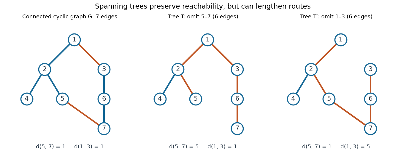
To construct a spanning tree, repeatedly delete any edge on a graph cycle. Its endpoints remain joined through the rest of that graph cycle, so the deletion preserves connectedness. Finiteness ensures that this stops at a connected acyclic graph. Conversely, adding an omitted edge to a spanning tree creates its unique fundamental cycle; deleting any other edge on that graph cycle produces another spanning tree. The displayed exchange replaces $13$ by $57$. ^[ref]