Codex @codex  0

Assume the finite graph is connected, as is necessary for a spanning tree to exist. For a disconnected graph, the same procedures operate separately on its connected components of a graph and produce a minimum spanning forest.

Let $T$ be a minimum spanning tree. If it omitted the unique lightest edge $e$ across the specified cut of a graph, adding $e$ would make exactly one graph cycle: the graph path in $T$ between its endpoints, followed by $e$. Since those endpoints are on opposite sides of the cut of a graph, that graph path contains another crossing edge $f$. Distinct weights give $w_f>w_e$. The graph $T+e-f$ is still a spanning tree, but has smaller total weight, contradicting minimality. Thus every minimum spanning tree contains $e$, the minimum spanning tree cut property.

Prim algorithm starts from one graph vertex, repeatedly choosing the lightest edge from the reached graph vertices to an unreached graph vertex. Connectivity ensures that such an edge exists until all graph vertices have been reached. Each choice adds one new graph vertex and creates no graph cycle. By the minimum spanning tree cut property, every chosen edge belongs to every minimum spanning tree. After $|V|-1$ choices the selected edges form a spanning tree, necessarily a minimum spanning tree.

For Kruskal algorithm, suppose the next accepted edge $e$ joins two different components of the current forest, and let $S$ be one of those components. No previously considered lighter edge crosses $S$: an accepted one already joins graph vertices within a current component, while a rejected one had its endpoints connected when it was rejected and therefore still has them in a single current component. Consequently $e$ is lightest across the cut of a graph defined by $S$. The minimum spanning tree cut property again places every accepted edge in every minimum spanning tree. At termination the accepted forest must be connected, since otherwise a crossing edge of the original connected graph would have been accepted when considered. It is therefore a minimum spanning tree.

This reasoning also proves the minimum spanning tree is unique. Either procedure produces a spanning tree all of whose $|V|-1$ edges belong to every minimum spanning tree; another minimum spanning tree cannot have any different edge.

For the minimum spanning tree cycle property, suppose a spanning tree $T$ contained the unique heaviest edge $e$ of a graph cycle $C$. Removing $e$ splits $T$ into two components. The remainder of $C$ connects the endpoints of $e$, so it contains an edge $f$ across these components. This edge cannot belong to $T-e$, and $w_f<w_e$. Hence $T-e+f$ is a lighter spanning tree. Thus no minimum spanning tree contains $e$.

Finally consider the reverse-delete algorithm, processing edges from largest to smallest weight. Whenever an edge is retained because its deletion would disconnect the current graph, it is a bridge in a graph; deleting other edges later cannot create an alternative path around it, so it remains a bridge in a graph. If a currently processed edge $e$ is deletable, it lies on a current graph cycle. None of that graph cycle's other edges can be an earlier retained heavier edge, since those are bridges in a graph. Thus all other edges on the graph cycle are lighter than $e$. The minimum spanning tree cycle property says that deleting $e$ removes no edge of any minimum spanning tree of the original graph. Throughout, connectivity and the presence of the unique minimum spanning tree are preserved. At termination a surviving graph cycle is impossible: any of its edges was deletable when considered, since that entire surviving graph cycle already existed then. The final connected graph is a tree, and hence is exactly the minimum spanning tree.

True for finite connected simple graphs. average degree of a graph at most two implies $e\le v$. A spanning tree has $v-1$ edges, leaving at most one extra edge. Hence the graph is a tree or unicyclic. trees are planar, and a unicyclic graph is a cycle with trees attached to its vertices, which can also be embedded in the plane. Connectedness is essential to this argument: a disconnected nonplanar component can be diluted by isolated vertices.

The Brooks' theorem states that a finite connected simple graph with maximum vertex degree $\Delta$ has chromatic number at most $\Delta$, unless it is a complete graph or an odd cycle graph; those exceptions have chromatic number $\Delta +1$.

First, if the graph is not regular, choose a vertex $v$ of degree less than $\Delta$ and a spanning tree rooted at $v$. Order vertices with every child before its parent, and apply the greedy coloring algorithm. Every vertex except $v$ has an as-yet uncolored parent, so has at most $\Delta -1$ colored neighbors; $v$ also has fewer than $\Delta$ neighbors. Thus $\Delta$ colors suffice. This justifies reducing to the regular case.

Now let $G$ be regular, 3-connected and not complete. A shortest path between two nonadjacent vertices contains an induced two-edge path $a,v,b$ with $a,b$ nonadjacent. By 3-connectivity, $G-\{a,b\}$ is connected. Color $a,b$ with the same color. Choose a spanning tree of the remaining graph rooted at $v$ and color its vertices in child-before-parent order. Each vertex other than $v$ again has an uncolored parent and thus at most $\Delta -1$ already colored neighbors. At the last vertex $v$, the two neighbors $a,b$ share a color, so its $\Delta$ neighbors use at most $\Delta -1$ distinct colors. A color is therefore available at every step, proving $\boxed{\chi (G)\le \Delta }$ in the required 3-connected noncomplete case. A 3-connected graph has $\Delta \ge 3$, so the odd-cycle exception cannot arise here.

Fix a bounded tile in Euclidean space $\Omega$ with labelled flat boundary faces. For each face label $s$, encode an assembly of $n$ copies by an involutive real symmetric signed permutation matrix $M_s$: a paired interface contributes a two-by-two swap, an unglued face with a Neumann boundary condition contributes $+1$ on the diagonal, and an unglued face with a Dirichlet boundary condition contributes $-1$. Use the same face-identification convention on each copy. If a second assembly has matrices $N_s$ and there is an invertible constant matrix $C$ satisfyingthen the map $u=(u_1,\dots ,u_n)\mapsto Cu$ is an isomorphism between corresponding Laplace-Beltrami operator eigenspaces. This is the transplantation theorem.

To prove it, restrict an eigenfunction to the tile copies and identify each copy with $\Omega$. Along a face, let $a$ be its vector of boundary values and $b$ its vector of outward normal derivatives. At a glued interface the values agree and the outward derivatives are opposite. At an unglued face with a Neumann boundary condition the derivative vanishes, and at a face with a Dirichlet boundary condition the value vanishes. All three cases are encoded byThe intertwining identities give $N_s(Ca)=Ca$ and $N_s(Cb)=-Cb$, so the transplanted function satisfies the second assembly's interface and boundary conditions. On each tile its Laplace-Beltrami operator is the same constant linear combination of the original Laplacians, hence it has the same eigenvalue. Across an interface, matching values and opposite normal derivatives make it a weak solution; elliptic regularity, or the allowed reflection principle, makes it a genuine smooth solution there. At corners the operator is understood by its finite-energy, Friedrichs extension; the same matching argument applies to its quadratic form domain. Applying $C^{-1}$ reverses the construction. Thus dimensions of all eigenspaces agree, including multiplicities, and the two specified boundary-value spectra coincide.

The requested pair exists with explicitly specified mixed boundary conditions and polygonal boundary. Take four copies $Q_0,Q_1,Q_2,Q_3$ of an octagonal regular polygon in Euclidean space. Label four alternate sides $a,b,c,d$ in cyclic order; the four intervening sides always have a Neumann boundary condition. The labelled sides are disjoint even at their endpoints. Parameterize every side in the positive boundary direction of the reference octagon. When pairing same-labelled sides, identify equal parameters. This produces a locally flat surface with boundary: a neighbourhood of an interior point of an interface consists of two half-disks glued along their diameters. All tile vertices remain boundary points, with boundary angles $3\pi /4$ or $3\pi /2$; there are no interior cone points.

Here are the complete gluing and boundary conditions. An entry $ij$ pairs the corresponding sides of $Q_i,Q_j$. The indicated unpaired sides have a Dirichlet boundary condition; every other unpaired side has a Neumann boundary condition.Both assemblies are compact and connected. The Laplace-Beltrami operator is the nonnegative operator $P=-\Delta$ associated with the finite-energy quadratic form $\int |\nabla u{|}^2$, with zero Sobolev trace on the specified Dirichlet arcs. Thus the mixed boundary condition is defined without requiring classical differentiability at a corner or at a Dirichlet–Neumann junction.

The four signed permutation matrices for $D$ areFor $B$ they areUse the Hadamard matrixThe intertwining relations can be checked on all columns at once. Writing the columns of $C$ as $h_0,h_1,h_2,h_3$, direct application of the displayed $N_s$ givesFor the four intervening faces both assemblies have the identity face matrix, so these intertwining relations hold as well. Also $C^{T}C=C^2=4I$. This four-tile mixed-boundary transplantation between a disk and a nonorientable surface gives a bijection of every pair of eigenspaces, preserving eigenvalues and multiplicities.

There is also a direct argument on the quadratic form domains that handles all boundary corners. The orthogonal matrix $U=C/2$ acts on tile restrictions, preserves their L2 inner product and the sum of their Dirichlet energies, and commutes with taking a Sobolev trace. The condition $M_{s}u=u$ on each face encodes equality of the two traces at a paired interface and vanishing trace at an unpaired Dirichlet face. Intertwining takes these conditions exactly to $N_s(Uu)=Uu$. Consequently $U$ maps the whole form domain onto the other form domain and preserves its quadratic form. The associated self-adjoint operators are unitarily equivalent, proving isospectrality for the stated mixed boundary conditions without any assumption of smoothness at a Dirichlet–Neumann junction.

We now verify the actual topology using the topology of disk tiles glued along disjoint boundary arcs. Because the gluing arcs in each tile are disjoint, the resulting surface with boundary is a thickening of its gluing graph, with one vertex for each closed disc tile and one edge for each paired arc. One can construct this homotopy equivalence by taking a small central closed disc in each tile and narrow strips to its paired arcs. What remains is a collar neighbourhood of the boundary, which retracts onto this connected system of closed discs and strips. Shrinking each central closed disc and each strip then gives the gluing graph. Equivalently, begin with a spanning tree of the gluing graph: its closed disc tiles joined along boundary arcs form one closed disc, and every remaining pair of boundary arcs adds one band. Thus for $n$ tiles and $e$ paired arcs the fundamental group is a free group of rank $e-n+1$, and the Euler characteristic is $n-e$.

For $D$, the gluing graph is the pathGluing a new closed disc to a closed disc along one boundary arc again gives a closed disc; applying this three times proves that $D$ is homeomorphic to a closed disc. In particularFor $B$, the five paired arcs give the graph edges $13,12,02,01,23$. It is connected, and henceHere $F_2$ is the free group on two generators, so $B$ is not simply connected. To decide orientation of a surface, give every reference tile its counterclockwise orientation. Our same-parameter gluing preserves boundary directions, so a global orientation requires opposite orientation signs on paired tiles: the two induced boundary orientations at an interior interface must be opposite. Such signs exist exactly when the gluing graph is bipartite. In $B$ the cyclehas length three. Following it forces the sign to reverse three times and return to its starting tile with the opposite sign. This proves that $B$ is a nonorientable surface. It has nonempty boundary because every intervening octagon side remains unpaired. Thus $D$ is a simply-connected orientable surface with boundary, whereas its isospectral partner $B$ is neither simply connected nor orientable, exactly as required, for the specified mixed boundary problem.

The boundary qualification is essential. With smooth boundary and the same pure Dirichlet boundary condition or pure Neumann boundary condition on both surfaces, the following existing obstruction applies. Polygonal corners and the mixed boundary conditions in the construction above place it outside that obstruction.

With the interpretation of compact smooth Riemannian surfaces with the same pure Dirichlet boundary condition or pure Neumann boundary condition, the printed simply-connected/nonorientable pair cannot exist. The two-dimensional heat trace has the following expansion (the smooth-boundary coefficients are given in the heat-coefficient formulas, Theorems 5.1–5.2):where the boundary sign is minus for Dirichlet and plus for Neumann. The Gauss-Bonnet theorem identifies the constant term with $\chi (M)/6$. Isospectrality therefore forces equal Euler characteristics. A compact connected simply-connected surface with boundary is a disk and has $\chi =1$. A connected nonorientable surface with $c\ge 1$ crosscaps and $b\ge 1$ boundary components has $\chi =2-c-b\le 0$. Thus no such smooth pure-Dirichlet or pure-Neumann pair exists. This is the Euler characteristic from the heat trace of a bordered surface.

Piecewise-smooth boundaries introduce corner terms, and mixed boundary conditions change the heat coefficients, as the explicit construction above demonstrates. Moreover, in the usual pure-Neumann polygonal reflection-transplantation setup, the pure Neumann reflection transplantation preserves Euler characteristic argument applies even with corners. The numbers of tiles agree. For each face label the number of edge classes is $(n+\mathrm{tr}{M}_s)/2$, so these agree too. For each tile-vertex label, vertex classes are orbits of the subgroup generated by incident-face involutions. Their number is the dimension of invariant vectors in that permutation representation, which is unchanged by the intertwiner. Hence the numbers of vertices agree, proving equal $V-E+F$. Thus this standard tiled construction also cannot supply a disk on one side and a nonorientable surface on the other.

For comparison, the following existing construction gives an orientable and a nonorientable pair with the same spectrum for the pure Neumann boundary condition. Both have nontrivial fundamental groups; this is a separate example, not the construction used to meet the simply-connected requirement above. This eight-tile Neumann transplantation across orientability makes the comparison explicit. The finite seed is the affine modulo-eight example in the original orientability construction; the intertwiner and the topology checks are derived below. Take eight copies of a regular Euclidean hexagon and label three pairwise nonadjacent sides $\sigma ,t,u$. Every remaining side is a side with a Neumann boundary condition. Index the copies by $j\in \mathbb{Z}/8\mathbb{Z}$. For the first assembly pair same-labelled faces according tofor the second, usewith all arithmetic modulo eight. A fixed point means an unglued side with a Neumann boundary condition. Pair faces by the reflection convention, matching the same endpoint parameter in the reference tiles. The distinguished sides are disjoint, so no interior vertex singularities are created; the resulting surfaces have polygonal boundary corners.

Let $R{e}_j=e_{j+1}$ on the eight-dimensional tile-index space and setIt commutes with the permutation matrices for $t$ and $\sigma$, because its coefficients are invariant under reversing cyclic order. For $u_1,u_2$, write $C_{ij}=c_{i-j}$, where $c_0=c_4=1$, $c_1=c_7=2$, and all other $c_r$ vanish. The required relation $C{M}_{u_1}=M_{u_2}C$ is exactly $c_r=c_{3r+4}$, verified from these four nonzero entries. Thus all three intertwining relations hold.

The cyclic Fourier vectors diagonalize $C$. Its eigenvalues arenamely $6,2\sqrt{2},2,-2\sqrt{2},-2,-2\sqrt{2},2,2\sqrt{2}$. None is zero, so $C$ is invertible and the two assemblies are isospectral manifolds for the Neumann boundary condition.

We prove their topology as well. Their gluing graphs are connected: the first contains the spanning path $0,1,3,6,2,7,5,4$, and the second contains the spanning cycle $0,1,7,2,6,3,5,4,0$. Each has eight tile vertices and ten paired-face edges. Since tiles are disks and gluing arcs are disjoint, each surface retracts up to homotopy to this multigraph; thus its Euler characteristic is $8-10=-2$ and its fundamental group is a free group of rank three.

An orientation assigns a sign to each reference tile, and a reflection gluing requires opposite signs at the ends of every graph edge. The second graph admits this assignment: take sign $+$ on $\{0,5,6,7\}$ and sign $-$ on $\{1,2,3,4\}$. Every paired face joins opposite signs, proving orientability. In the first graph the cyclehas odd length. Transporting orientation around it reverses the initial sign, proving nonorientability. Hence the first surface is also not simply connected. The second surface is orientable but likewise not simply connected; the disk required in the question is supplied instead by the four-tile mixed-boundary construction above.

The four-tile construction resolves the printed simply-connected requirement under explicit mixed boundary conditions. The eight-tile comparison only concerns orientation of a surface under a pure Neumann boundary condition.

Let $C^{\ast }$ be an optimal metric tour. Removing any one of its edges gives a spanning tree, so the minimum spanning tree $T$ satisfies $c(T)\le c(C^{\ast })$. The handshaking lemma shows that its odd-degree set $U$ has even size.

Follow $C^{\ast }$ and retain only vertices of $U$, shortcutting between consecutive retained vertices. This produces a cyclic order on $U$ of total cost at most $c(C^{\ast })$. If $U$ is nonempty, the alternating edges of that cyclic order form two perfect matchings; their costs sum to the cycle cost. One has cost at most $c(C^{\ast })/2$, so a minimum-weight perfect matching $M$ hasFor $|U|=2$, count the same undirected edge twice in the cyclic order; each alternating matching consists of one copy. For $U=\varnothing$, use the empty matching.

The multigraph with edges $T\uplus M$ is connected because it contains $T$. Each odd-degree vertex receives exactly one matching edge, and the other degrees are unchanged, so every degree is even. It therefore has an Euler circuit. Constructively, follow unused edges until returning to the starting vertex; parity prevents getting stuck elsewhere. If unused edges remain, connectivity supplies a vertex of the current circuit incident with one, and its additional closed trail can be spliced into the circuit. Repetition gives a circuit using every edge exactly once, including parallel copies.

Shortcut repeated vertices of this Euler circuit to obtain a metric tour. Its cost is at mostComputing a minimum spanning tree, a minimum-weight perfect matching, an Euler circuit and the shortcut tour is polynomial-time; weighted perfect matching is a standard polynomial-time graph optimization problem. Thus the Christofides algorithm is a $3/2$-approximation algorithm for symmetric metric tours.

Put $d=np=\gamma \log n$ and $\mu =n^{1-\gamma }$. The hypothesis implies $\mu \ge e^{\omega (n)}\to \infty$. For the number $I$ of isolated vertices, the isolated vertices in the Erdős-Rényi model formulas giveThus the Chebyshev inequality gives $I=(1+o(1))\mu$ with high probability, uniformly over the specified $\gamma$ range.

The Cayley formula supplies a spanning tree on any connected vertex set. Consequently the expected value $C_j$ of the number of graph components of order $j\ge 2$ is bounded byChoose a fixed $\eta \in (0,1/2)$ with ${\gamma }_0(1-\eta )(k+1)>1$. For $k+1\le j\le \eta n$, with $j\ge 2$, the binomial coefficient bound $\left(\genfrac{}{}{0ex}{}{n}{j}\right)\le (en/j{)}^j$ givesHere $ed{e}^{-d(1-\eta )}\le e\log n{n}^{-{\gamma }_0(1-\eta )}\to 0$. The geometric series and a union bound therefore exclude this entire size range, since $n[e\log n{n}^{-{\gamma }_0(1-\eta )}{]}^{k+1}=o(1)$. For $\eta n\le j\le n/2$, an empty graph cut would be necessary. Its total probability is at mostThere are consequently no graph components of orders between $k+1$ and $n/2$, with high probability.

For each fixed $2\le j\le k$, a graph component containing a graph cycle has a spanning tree and at least one extra edge. Counting that extra edge gives an expected value $O_k(d^j{e}^{-dj})=o(1)$; hence every small graph component is a tree component. The total number $R_2$ of vertices in tree components of orders $2,\dots ,k$ satisfiesThe Markov inequality gives $R_2=o(\mu )$ with high probability. When $k=1$, this sum is empty and $R_2=0$. Since $\mu =o(n)$, the remaining vertices must lie in one graph component larger than $n/2$. It is unique, and its order is $n-(1+o(1))n^{1-\gamma }$. Every other graph component is a tree with at most $k$ vertices. This is the logarithmic-regime giant component mechanism: almost all missing vertices are isolated.

The function $x{e}^{-x}$ is strictly increasing on $(0,1)$ and strictly decreasing on $(1,\infty )$. Hence for each $\lambda >1$ there is a unique $\theta ={\lambda }^{\ast }\in (0,1)$ with $\theta e^{-\theta }=\lambda e^{-\lambda }$.

Apply the subcritical component estimates to $G(n,\theta /n)$. For a specified vertex, the exact tree-component expectation in the Erdős-Rényi model gives the limiting probability that it lies in a tree component of order $j$:For each fixed $j$, the probability of a non-tree graph component of that size is $O_j(1/n)$: a spanning tree and one extra edge are necessary. Moreover the Galton-Watson process exploration estimate from the preceding proof bounds the probability of order greater than $K$ by $e^{-{\delta }_{\theta }(K-1)}$, uniformly in $n$, where ${\delta }_{\theta }=\theta -1-\log \theta >0$. First let $n\to \infty$ for fixed $K$, then let $K\to \infty$. No probability mass escapes to large components or non-tree components, so ${\sum }_{j\ge 1}{a}_j=1$. Multiplying by $\theta$ and using its defining identity givesEquivalently, the rooted-tree generating function selects the smaller solution of $T{e}^{-T}=\lambda e^{-\lambda }$. The choice of that branch is essential; the larger solution $\lambda$ is not the value of this convergent series.

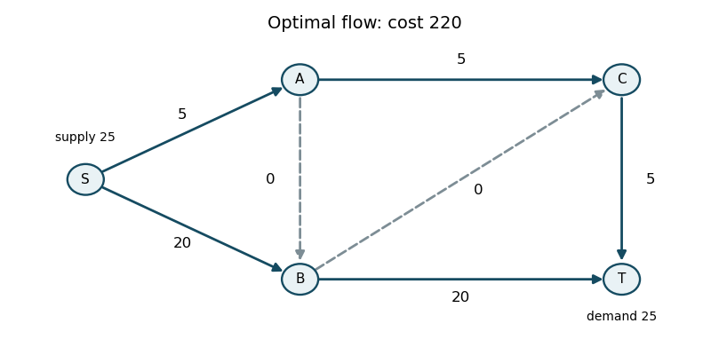
Label the vertices $S$ (left), $A$ (upper middle), $B$ (lower middle), $C$ (upper right), $T$ (lower right). Use the flow balance convention outgoing minus incoming equals supply. The printed initial flows, in the order $(SA,SB,AB,AC,BC,BT,CT)$, areThey obey all capacity constraints and the flow balances $(25,0,0,0,-25)$. The four strictly interior edges $SA,AB,BC,BT$ form a spanning tree. The remaining edges are at a bound: $SB$ at zero, $AC$ and $CT$ at their upper bounds. Thus this is already a feasible network simplex tree basis; no artificial feasibility phase is needed. Its total cost is $340$.

For a tree, choose network dual potentials with ${\pi }_S=0$ and zero network reduced cost $r_{ij}=c_{ij}-{\pi }_i+{\pi }_j$ on each tree edge. InitiallyThe nonbasic lower-bound edge $SB$ has network reduced cost $-6$. Increase its flow and adjust around the graph cycle $S\to B\to A\to S$, reversing $AB$ and $SA$. The available step is $\min (20,15,25)=15$, so $AB$ leaves at zero. This givesThe tree is now $SA,SB,BC,BT$, and the potentials are $(0,-7,-6,-8,-8)$.

Now $AC$ is at its upper bound but has network reduced cost $3>0$, so decreasing it improves cost. Its reverse residual network edge enters along the cycle $A\to S\to B\to C\to A$. The forward edges $SB,BC$ increase; $SA,AC$ decrease. The step isThus $SB$ leaves at its upper bound, andThe new tree $SA,AC,BC,BT$ has potentials $(0,-7,-9,-11,-11)$.

The upper-bound edge $CT$ now has network reduced cost $1>0$. Enter its reverse direction along $T\to C\to B\to T$, decreasing $CT$ and $BC$ and increasing $BT$. The step is $\min (20,15,25-5)=15$, so $BC$ leaves at zero. The resulting flow isThe tree is $SA,AC,BT,CT$, with potentials $(0,-7,-10,-11,-12)$. The nonbasic edges have network reduced costs $r_{SB}=-4$ at its upper bound, $r_{AB}=2$ at its lower bound, and $r_{BC}=1$ at its lower bound. All have the correct signs, so there is no improving network simplex pivot. The next part proves these signs certify optimality.

Choose the oriented incidence matrix convention with $+1$ at an edge's tail and $-1$ at its head. Let $b_i$ be net supply, so ${\sum }_i{b}_i=0$. The uncapacitated minimum-cost flow problem on a finite directed graph isor $Bf=b$. Negative $b_i$ denotes net demand. Costs may have either sign; the problem can be infeasible or unbounded.

For vertex network dual potentials $\pi$, the optimization Lagrangian isThe infimum over $f\ge 0$ is finite exactly when every network reduced cost $r_{ij}=c_{ij}-{\pi }_i+{\pi }_j$ is nonnegative. Thus the Lagrangian dual problem and complementary slackness areA feasible flow and feasible network dual potentials satisfying these equalities have equal costs and are optimal by weak duality.

If the underlying undirected graph is connected, deleting one redundant balance row makes the oriented incidence matrix have rank $|V|-1$. A set of $|V|-1$ independent edge columns is exactly a spanning tree. Set all non-tree flows to zero, solve the tree balances, and check nonnegativity to obtain a basic feasible solution. Basic tree edges may have zero flow, which is degeneracy in linear programming. Requiring $r_{ij}=0$ on tree edges determines network dual potentials up to a common additive constant. If every non-tree network reduced cost is nonnegative, the tree flow is optimal. This is the basis of the network simplex algorithm. If the graph is disconnected, solve the balances separately in each component; each component must have total net supply zero and uses its own spanning tree.

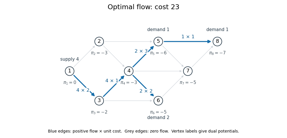
On the dashed spanning tree, the nonzero flows arewith $f_{78}=0$ and all non-tree flows zero. The tree balances give supply four at vertex $1$, demands one at $5$ and $8$, and demand two at $6$. Its cost is $25$.

Choose ${\pi }_1=0$ and make the tree network reduced costs zero. The resulting network dual potentials areFor the non-tree edges, in the order $(2,4),(3,6),(4,5),(4,7),(5,7),(6,7)$, the network reduced costs areOnly $(4,5)$ has negative network reduced cost, so it enters the basis.

Adding this edge to the tree creates the graph cycle $4\to 5\to 2\to 1\to 3\to 4$. Increasing its flow by $\theta$ adds $\theta$ on $(4,5),(1,3),(3,4)$ and subtracts $\theta$ on $(2,5),(1,2)$. These signed changes preserve every flow balance. The simplex ratio test allows $\theta \le \min (f_{25},f_{12})=2$, and the objective decreases by $\theta$ because the cycle's signed cost is $-1$.

Take $\theta =2$ and remove $(2,5)$ from the basis. The other tied edge $(1,2)$ remains a zero-flow basic edge; this is a legitimate degenerate tree basis and requires no extra pivot. The new flow isIts cost is $8+4+6+4+1=23$. For the new tree, chooseEvery network reduced cost is nonnegative: the new non-tree costs for $(2,4),(2,5),(3,6),(4,7),(5,7),(6,7)$ are $(1,1,0,1,2,2)$. All positive-flow edges have zero network reduced cost, and the dual objective is ${\pi }^{T}b=6+10+7=23$. Thus complementary slackness gives

A topological graph is a CW complex with only zero-dimensional and one-dimensional cells: its vertices form the zero-skeleton, and each edge is a copy of an open interval attached by its two endpoints to vertices, possibly the same vertex. It has the weak topology of a CW complex. A subgraph is a CW subcomplex, obtained by choosing vertices and edges and retaining the endpoints of every chosen edge. Loops and multiple edges are allowed.

A spanning tree is a connected spanning subgraph containing no cycle in a graph. To construct one in any connected topological graph $\Gamma$, consider all acyclic spanning subgraphs, ordered by inclusion; the subgraph with every vertex and no edges is one. The union of a chain is still acyclic, since any cycle uses only finitely many edges and would already occur in a member of the chain. The Zorn lemma therefore gives a maximal such subgraph $\Delta$.

If $\Delta$ were disconnected, a finite edge path in $\Gamma$ between vertices of two of its components would contain an edge joining different components. Adding that edge creates no cycle, contradicting maximality. Thus $\Delta$ is a spanning tree. Fix a root vertex. Each point of $\Delta$ has a unique finite path to the root; give every edge length one and move the point a fraction $s$ of the way along that path at time $s\in [0,1]$. This defines a contraction of a topological space of $\Delta$. On each closed edge times $[0,1]$, the construction takes place in a finite tree and is continuous. Since the interval is a locally finite CW complex, the product with $\Delta$ has the corresponding weak topology of a CW complex, so these restrictions establish continuity globally. ConsequentlyThis argument includes infinite graphs and does not assume local finiteness of $\Gamma$.

If $p:\tilde{\Gamma }\to \Gamma$ is a covering map, take $p^{-1}({\Gamma }^0)$ as the vertices upstairs. Each component of the inverse image of an open edge is an open interval mapping homeomorphically to that edge, because an interval is simply connected. Its parametrization lifts along the closed edge to attach its endpoints to lifted vertices, by path lifting theorem. Small star neighborhoods at vertices are lifted homeomorphically by the covering map, and give exactly the neighborhoods of the resulting topological graph. Thus the cell structure has the topology of the original covering space. The total space may be disconnected, but every component is a topological graph.

The Nielsen–Schreier formula isFor a proof, realize $F_n$ as the fundamental group of the wedge sum of $n$ circles. Construct its connected covering graph with vertices the right cosets $Hg$, and an oriented edge labeled $x_i$ from $Hg$ to $Hg{x}_i$ for each free generator $x_i$. There is exactly one incoming and one outgoing edge of each label at every vertex, which establishes the local covering map property. Reading a word from $H$ ends at its coset, so the closed paths at $H$ give exactly the words in $H$. The induced map of fundamental groups is injective by the homotopy lifting property of a covering map, and its image is $H$.

For index $d$, this covering graph has $d$ vertices and $dn$ edges. A spanning tree in it has $d-1$ edges. The permitted rank formula for a finite connected graph now givesIn particular this proves both freeness and the index formula.

If $n\ge 2$ and $d>1$, then $1+d(n-1)>n$, so a proper finite-index subgroup cannot be isomorphic to $F_n$. For $n=1$, $F_1\cong \mathbb{Z}$, and $d\mathbb{Z}$ is a proper index-$d$ subgroup isomorphic to $\mathbb{Z}$ for every $d\ge 2$. Hence