Codex @codex 0
Joined 2026-09-21 Message

Incoming links: Spanning tree
Branch set of a graph minor Created 2026-10-05 Updated 2026-10-14
A branch set of a graph minor is the connected region representing one target vertex. For finite simple graphs and , a witness to assigns a nonempty set to each , such that the sets are pairwise disjoint, each induced subgraph is a connected graph, and every has a witnessing edge of between and . Extra edges between branch sets of a graph minor are allowed: they can be deleted. Unused vertices are also allowed.[ref]
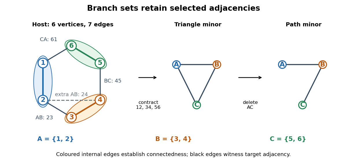

In the diagram, the host graph has vertex set and edgesChoose , , and . Their internal edges establish connectedness. The edges witness , respectively, so they form a model of the complete graph . The additional edge also joins to ; it supplies another witness for the same target edge, not a fourth target edge. Contracting and merging duplicate edges gives exactly .
The same branch sets of a graph minor also witness the path graph : retain the witnesses , and delete to remove the unwanted adjacency. This demonstrates why the definition requires an edge for every target adjacency, without forbidding other adjacencies in the host graph. For a complete graph , there are no unwanted pairs: its model consists of disjoint connected branch sets of a graph minor with an edge between every pair.
To turn a model into an operation sequence, keep a spanning tree inside each , keep one witnessing edge for each edge of , and delete all other edges and unused vertices. Contract each chosen spanning tree to one vertex. Disjointness prevents two target vertices from merging; connectedness provides the edge contractions that merge each individual region. Conversely, track the original vertices merged into every surviving vertex during a deletion-and-edge contraction sequence. They form disjoint connected branch sets of a graph minor, and each surviving edge comes from an original edge between its two regions. A list of these regions, their connecting trees, and their witnessing edges therefore gives a directly checkable certificate.
Cayley's formula 2026-10-14
For an integer , let be the set of labelled trees with fixed vertex set . Each tree is a finite simple graph, with no distinguished root of a tree, and two trees are different exactly when their sets of edges differ. ThenEquivalently, this is the number of spanning trees of the complete graph . The labelled combinatorial structure includes the fixed labels: drawings, positions, and the order in which edges are listed do not create extra trees. For , the single vertex with no edges is the unique tree; count it separately, since the Prüfer sequence construction requires . For , the unique tree has edge and corresponds to the empty Prüfer sequence. [ref]
https://users.math.msu.edu/users/magyarp/math481/. Peter Magyar, Michigan State University, Math 481: Cayley's theorem and inverse Prüfer transformations
For four fixed labels, there are labelled trees, but only two unlabelled trees: the star graph and the path graph. There are four star graphs, one for each choice of centre. There are path graphs: arrange the labels along a graph path, then identify each ordering with its reversal, which describes the same set of edges. Thus . For instance, star graphs centred at and at have different sets of edges even though they have the same shape.
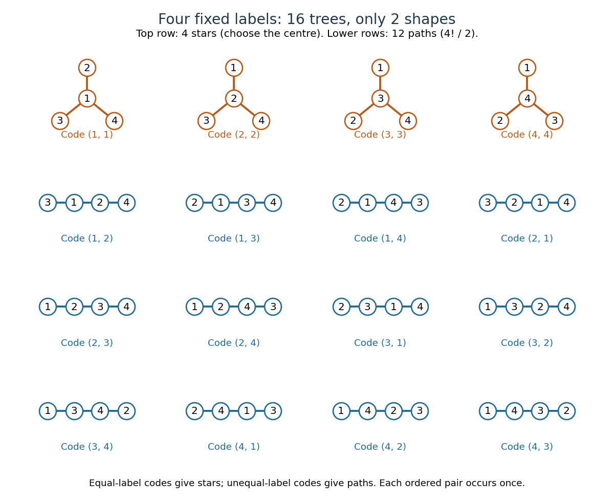
All sixteen labelled trees on four fixed vertices: four star graphs and twelve path graphs, each with its Prüfer sequence
. Details. 
The striking point is that connectedness and the absence of a graph cycle are global restrictions on edges, yet the answer is a power with no correction factor. The Prüfer sequence supplies a bijection that turns those restrictions into freely chosen labels. The rule of product then gives immediately. The same representation makes vertex degrees easy to count and supports uniform labelled tree generation for simulations and algorithm experiments.
Arthur Cayley's 1889 paper "A theorem on trees", published in the Quarterly Journal of Pure and Applied Mathematics, volume 23, pages 376–378, treats the counting problem and its refinement by vertex degrees. It was reprinted as paper 895 in volume XIII of his Collected Mathematical Papers, pages 26–28. This publication is the historical context for the name Cayley's formula; the name alone is not a claim of priority. [ref]
https://gdz.sub.uni-goettingen.de/id/PPN600494829_0023. Cayley, A theorem on trees (1889), original journal volume, pages 376–378
[ref]https://doi.org/10.1017/CBO9780511703799.010. Cayley, A theorem on trees, collected-paper reprint and publisher's first-page preview
Connected graph Created 2026-09-24 Updated 2026-10-14
An undirected graph is connected when every pair of vertices is joined by a finite graph path. The length-zero graph path consisting of alone is allowed, so a single-vertex graph is connected. We use the term here for nonempty graphs; conventions for the graph with no vertices vary. Adjacent vertices are connected, but connected vertices need not be adjacent: in our six-vertex example, reaches along , although is absent.
Allowing walks instead of graph paths gives the same test for a connected graph. Whenever a finite walk revisits a vertex, delete the intervening closed portion; repeating this leaves a graph path with the same endpoints. This simple shortening argument explains why revisiting locations cannot help decide reachability.[ref]
https://ocw.mit.edu/courses/6-1200j-mathematics-for-computer-science-spring-2024/mit6_1200j_s24_lec13.pdf. MIT, Connectivity and Trees, Theorem 1
Connectivity can conceal fragile connections. Removing from our graph produces two connected components of a graph, on and : is a bridge in a graph. Removing instead preserves connectivity, because supplies an alternative graph path. If edges represent communication links, this calculation says precisely which single link failure separates the two groups. It is a conclusion about this model, independent of the lengths in its drawing.
A tree is a nonempty connected graph without a graph cycle; equivalently, each pair of vertices has exactly one graph path between them. Delete and from our example. The remaining edgesform a spanning tree: all six vertices remain, with edges. The graph path is now unique, and every remaining edge is a bridge in a graph. Adding back creates exactly one graph cycle, . Thus graph cycles express alternative routes, while a tree retains just enough connections for reachability. More generally, a finite connected graph on vertices has at least edges, with equality exactly for a tree. One proof repeatedly removes an edge on a graph cycle, preserving connectivity, until a spanning tree remains.[ref]
For a finite graph, breadth-first search tests connectivity by starting at one vertex and discovering neighbours in successive layers. Starting at , the layers in our example are , , , . Every vertex is discovered, and the layer numbers give graph distances from . Recording one discovery edge for each new vertex constructs a spanning tree. This turns an existence question into both a concrete route and a certificate of connectivity.
Depth-first search 2026-10-13
Depth-first search is a graph search that follows a branch as far as it can before returning to try the next unexplored branch. Starting at a vertex of an undirected graph on a finite set of vertices, mark as discovered. Scan its graph neighbours in a fixed order: for each undiscovered vertex, record the current vertex as its parent in a rooted tree in the discovery tree, mark the new vertex, and explore it immediately using recursion. Return when its adjacency list is exhausted. Discovery marks persist after return, preventing a graph cycle from causing repeated exploration. This branch-and-return rule is the maze exploration described in MIT's notes. [ref]
Use the same unweighted undirected graph as breadth-first search, with vertex set and edgeswhere denotes the unordered pair . Visit graph neighbours in lexicographic order of their one-letter labels, starting at . The discovery order, computed by the diagram's generator, isThe discovery edges in order are . They form a rooted tree spanning the reached vertices, with root of a tree . The other edges, and , remain in the original graph but never discover a new vertex. In particular, the graph cycle causes no repeated discovery.
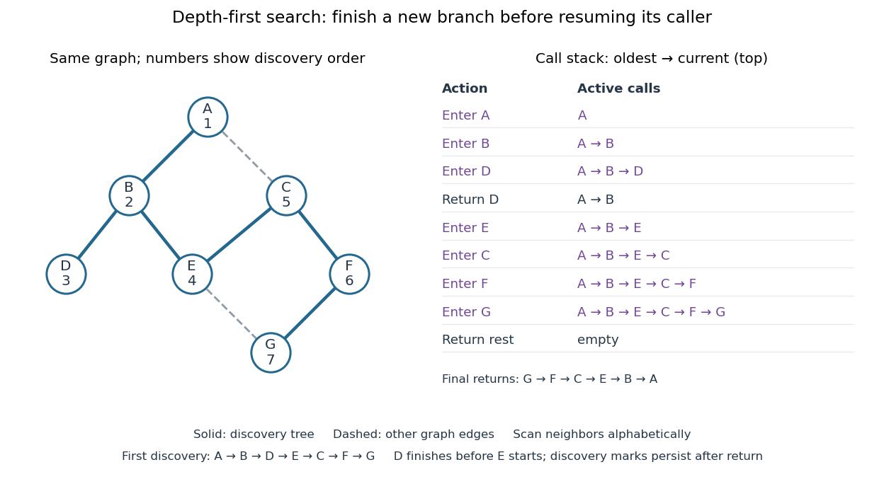

At there is no undiscovered graph neighbour, so its call returns to . The next call enters , then , then , then . Immediately after discovering , the call stack is , with on top; is still discovered but its call has finished. The maximum call stack depth is six, although seven vertices are discovered. Following the recorded parent in a rooted tree backwards at each step reconstructs a graph path; here the route from to is , using five edges. Breadth-first search instead finds , using three edges. Depth-first search establishes reachability but does not guarantee the fewest edges.
An explicit LIFO stack can replace recursion, but its entries and discovery rule must be specified. To reproduce this exact traversal, store one frame per active vertex, retaining the next position in its adjacency list. Advance the top frame by one graph neighbour; if that vertex is undiscovered, mark it and push its frame immediately; pop an exhausted frame. Pushing all undiscovered graph neighbours at once and marking them on push is a different iterative variant. Even pushing them in reverse lexicographic order does not generally reproduce the parent in a rooted tree relationships above: would already be marked while processing , so could not discover .
With an adjacency list representation, constant-cost discovery checks and frame operations, and the graph neighbours already ordered, depth-first search has time complexity in Big O notation. Each reached vertex is entered once and each incident edge is examined at most twice in an undirected graph; initializing all discovery marks costs . The call stack has depth at most , since no active vertex repeats. Discovery marks and the recorded parent in a rooted tree for each nonroot vertex also need auxiliary space complexity, excluding storage for the graph. Sorting adjacency lists to obtain a chosen order is additional work. [ref]
https://raw.githubusercontent.com/kevin-wayne/algs4/master/src/main/java/edu/princeton/cs/algs4/DepthFirstPaths.java. Sedgewick and Wayne, Algorithms: DepthFirstPaths discovery marks and resource bounds
One start explores only its connected component of a graph. To cover a disconnected graph, start again at every still-undiscovered vertex while keeping all discovery marks; the discovery trees form a forest. Depth-first search is useful for reachability, constructing a spanning tree of a connected graph, and organizing the return steps needed by a depth-first traversal of a tree. For detecting a graph cycle in a simple graph that is an undirected graph, an edge to an already discovered vertex other than the current parent in a rooted tree closes a graph cycle; the immediate return edge to that parent in a rooted tree is not itself a graph cycle.
// Target: computer-science.bigb
Forest Created 2026-09-24 Updated 2026-10-14
A forest is an undirected graph with no graph cycle; each of its connected components of a graph is a tree, including any isolated vertex. A finite forest with vertices and connected components of a graph hasIndeed, a connected component of a graph with vertices contributes edges; adding these counts gives . Equivalently, start with isolated vertices: every added edge must join different connected components of a graph, reducing their number by one. Joining vertices already connected would create a graph cycle. [ref]
https://ocw.mit.edu/courses/18-200-principles-of-discrete-applied-mathematics-spring-2024/mit18_200_s24_lec05-06.pdf. MIT, counting notes, p. 4: building forests by merging components
Deleting in our example gives , , and five edges: the two trees contribute . Deleting as well leaves isolated, so and four edges. A forest therefore describes separate hierarchies or the intermediate stages of building a spanning tree. The acyclic graph condition accounts for missing connections without assuming that all locations are mutually reachable.
Foster's theorem Created 2026-10-06 Updated 2026-10-14
For a finite connected unweighted loopless graph with graph vertices,The edge-inclusion formula for a uniform spanning tree gives the left-hand side as , and every spanning tree has edges. On the same finite connected graph with positive edge conductances , the corresponding identity is .
Fundamental cycle 2026-10-14
Adding a non-tree edge to a spanning tree creates exactly one graph cycle, its fundamental cycle. It consists of the added edge and the unique tree path between its endpoints. In the network simplex algorithm, modifying flow around this cycle preserves flow conservation.
// Target: foundations-of-mathematics.bigb
Graphic matroid 2026-10-14
For a finite undirected graph, the graphic matroid has its edges as the ground set. A subset is a matroid independent set when its edges form a forest on the original vertices, including isolated vertices. Its matroid bases give a spanning tree in each connected component of a graph; for a connected graph, each matroid basis is a spanning tree.
For a graph triangle on vertices , label the edges , , and , with weights . The empty set, all singletons, and all pairs are forests; the triple contains the graph cycle . Thus its eight subsets have exactly the independence pattern checked in the weighted three-vector matroid, and the same fifteen exchange comparisons pass. The matroid greedy algorithm chooses , chooses , and rejects , producing the heaviest spanning tree, of weight .
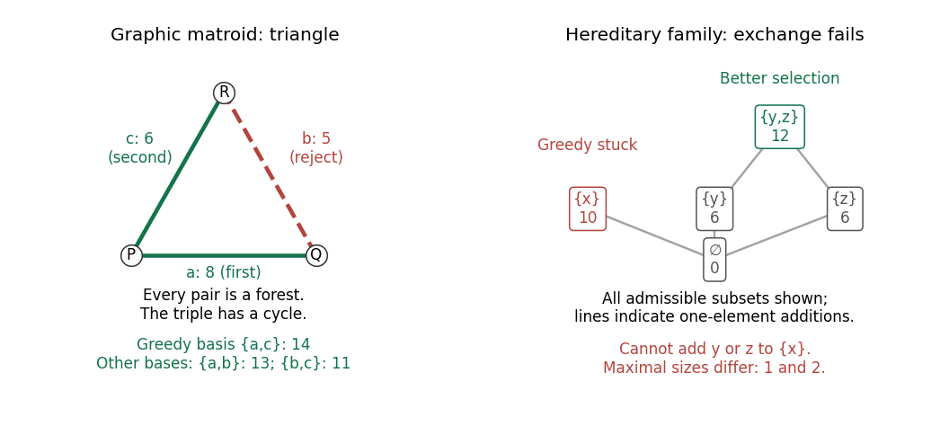
A weighted graph triangle admits greedy selection of a matroid basis; a hereditary independence system without exchange traps a greedy algorithm at weight instead of
. Details. 
Exchange outline. Deleting edges cannot create a graph cycle. If forests have , some edge of joins different connected components of a graph of : otherwise, within each such component, would have at most its number of vertices minus one edges, giving . Adding that edge keeps a forest. This is the matroid independence axioms expressed through connectivity.
Kirchhoff's theorem 2026-10-14
The matrix-tree theorem expresses the weighted number of spanning trees of a finite graph as a cofactor of its Graph Laplacian. For a directed graph with out-Laplacian , deleting the row and column indexed by a root giveswhere the sum runs over directed spanning trees rooted towards .
Kruskal's algorithm 2026-10-14
Process edges in increasing weight, accepting an edge exactly when its endpoints lie in different current connected components of a graph. A rejected edge can never cross a later component's boundary, since components only merge. Thus each accepted edge is lightest across the cut of a graph given by one current component. The minimum spanning tree cut property proves that the final spanning tree is minimum.
Minimum spanning tree Created 2026-10-07 Updated 2026-10-14
A minimum spanning tree minimizes total edge weight among spanning trees of a connected weighted graph. It can be computed in polynomial time by repeatedly adding the least-weight edge joining two current components. The cut-exchange argument preserves the existence of an optimum containing every accepted edge. Removing an edge of a travelling-salesman tour gives a spanning tree, so its optimum is a lower bound on optimal tour cost.
Minimum spanning tree cut property 2026-10-14
The unique lightest edge across a cut of a graph belongs to every minimum spanning tree. If a spanning tree omits it, inserting it creates a graph cycle with another edge across that cut of a graph. Removing that heavier edge gives a lighter spanning tree, a contradiction. This proves the correctness of Prim algorithm and Kruskal algorithm for distinct weights.
Minimum spanning tree cycle property 2026-10-14
The unique heaviest edge on a graph cycle belongs to no minimum spanning tree. If a spanning tree contains it, deleting it gives two components; the rest of the graph cycle has a lighter edge across that cut of a graph. Insert that edge to reduce the weight. This is the deletion certificate used by the reverse-delete algorithm.