Assignment of observations to categories using measured features and a statistical rule. In geological remote sensing, features can be multispectral pixel values or derived spectral reflectance ratios; known field samples provide training labels and independent observations assess errors. Classification boundaries need not coincide with lithological contacts when illumination or cover dominates the signal.
Within-observer agreement versus reference agreement distinguishes consistency of an observer's repeated labels from concordance with a separately defined reference. The first asks whether the observer repeats a decision; the second asks whether that decision matches the comparison standard. In statistical classification, neither quantity can replace the other.
For cases, let and be one observer's labels at two readings, and the reference label. Define the two empirical agreement fractionsAn original binary example has 100 cases, half reference-positive and half reference-negative. An observer reverses every reference label and repeats that reversal on the second reading. Then while . Perfect repeat agreement can coexist with complete reference disagreement. An observer always assigning the negative label also has perfect repeat agreement, but only 50 percent reference agreement in this balanced example.
A confusion matrix shows which categories contribute to disagreement, whereas a single overall percentage can conceal systematic shifts or an imbalanced case mix. Reference agreement is classification accuracy relative to that reference, not proof that the reference is infallible. A consensus panel, a later outcome and an independent molecular test answer different validation questions.
A primary 2017 study made this distinction experimentally by having pathologists interpret skin-biopsy sets twice, at least eight months apart, and comparing their interpretations with an experienced consensus reference. The study started with 240 cases and reported reproducibility separately from reference concordance.[ref]
Pathologists' diagnosis of invasive melanoma and melanocytic proliferations: observer accuracy and reproducibility study by Joann G. Elmore and others. BMJ 357, j2813, Abstract, Participants and outcome definitions
The delayed repeat reduced immediate recall, but did not transform repeated judgments into independent biological truths.A useful evaluation preserves case identity, reading order and the exact reference procedure. If a machine learning classifier learns an observer's systematically shifted labels, it may reproduce that observer well while disagreeing with the external reference. Reporting both comparisons makes that limitation visible. Uncertainty estimates should also account for repeated cases and multiple readings rather than counting every label as an independent subject.
Probability calibration means that reported probabilities agree with the frequencies of the outcomes they describe. For binary classification, let be the true label and let be the predicted positive-class probability. Population calibration is the conditional expectation conditionAmong cases receiving a value near , the positive fraction should therefore be near , with uncertainty in any finite sample.[ref]
Probability calibration in the scikit-learn documentation. Opening definition and section 1.16.1: binary probabilities and observed positive fractions
A simple example separates calibration from discrimination. Suppose the population has a positive fraction of and a predictor always reports . Then , so it is calibrated, although it cannot rank one case above another. Conversely, replacing a useful score by a strictly increasing transformation such as preserves ranking but generally changes the claimed probability. Thus ordering cases and attaching reliable numerical probabilities are different tasks.
A reliability diagram estimates the agreement by grouping predictions and comparing each group's mean prediction with its observed outcomes. Assess it using suitable held-out observations. A calibrator fitted to predictions on the same observations used to fit the original model can inherit an overly optimistic picture of performance; fitting and evaluation need appropriate separation.[ref]
A 2017 study found substantial confidence miscalibration in the evaluated neural networks, even when prediction accuracy improved. It also tested temperature scaling as a compact post-processing adjustment. These were empirical results on specified models and datasets, rather than a theorem that all neural networks are miscalibrated.[ref]
On Calibration of Modern Neural Networks by Chuan Guo and others. Figure 1 and sections 3–4: experimental comparisons and calibration methods
Expected calibration error summarizes how reported confidence differs from observed correctness. For top-label statistical classification, the population quantity compares correctness probability conditional on confidence with that confidence. A commonly reported finite-sample estimate groups predictions into confidence intervals and compares the mean confidence and accuracy in each interval.[ref]
On Calibration of Modern Neural Networks by Chuan Guo and others. §2, Eqs. (2)–(3), population calibration gap and binned estimate
For a nonempty bin among predictions, defineHere is confidence in the selected class, not its numerical label. The empirical statistic isEmpty bins have zero weight and need no undefined bin average. The cited paper uses equal-width bins.[ref]
On Calibration of Modern Neural Networks by Chuan Guo and others. §2, bin definitions and Eq. (3), printed pp.1322–1323
A synthetic example shows why the partition matters. Four predictions have confidences and correctness indicators . With one bin, accuracy and mean confidence are both , so the estimate is zero. With four equal-width bins on , only the last two are populated. Their accuracy/confidence pairs are and , each with half the observations. ThusThis is ten percentage points, despite unchanged predictions and labels.
A zero coarse-bin result can conceal opposing gaps; it does not establish perfect probability calibration or agreement within every subgroup. Report bin boundaries, sample size, confidence convention and scale. Reliability diagrams reveal where the gaps occur, while a scalar expected calibration error supplies their sample-weighted summary. It is distinct from the fraction of incorrect classifications.
Temperature scaling is a method of probability calibration that divides a model's neural network logits by one fitted positive scalar before applying the softmax function. The temperature is selected after model training, using labels in a held-out validation set to minimize the negative log-likelihood. It adjusts reported probabilities without retraining all model weights.[ref]
On Calibration of Modern Neural Networks by Chuan Guo and others. §4.2, Eq. (9), scalar temperature and validation negative log likelihood
For class scores and ,For the synthetic two-class scores , the first-class probability isThe selected class remains the first while its reported confidence decreases.
The preservation of the selected class follows directly: dividing by positive preserves every score ordering and equality, and exponentiation is strictly increasing. Thus the set of classes attaining the largest score is unchanged. This concerns ordering between classes within one example; it does not assert preservation of confidence ordering between different examples.
A motivating measurement in the original study compares reliability diagrams for a 110-layer image-classification network. Its reported expected calibration error changes from before calibration to after temperature scaling. This is a result for that experimental setup and binned metric, not a guarantee for every classifier or input distribution.[ref]
On Calibration of Modern Neural Networks by Chuan Guo and others. §5 and Fig. 4, CIFAR-100 ResNet-110 before/after reliability diagrams
Use separate data for fitting the temperature and for final evaluation. One scalar can improve an overall confidence mismatch but cannot represent every class-specific or input-dependent error. The name refers to this probability transformation; no physical temperature is being measured.
A reliability diagram compares predicted probabilities with observed outcome frequencies to assess probability calibration. For the positive-class version of binary classification, partition observations into bins according to their predicted probabilities . For every nonempty bin, plotwhere is for a positive outcome and otherwise. Agreement places the estimated points near the diagonal . Empty bins have no observed fraction and should not be plotted as zero.[ref]
Probability calibration in the scikit-learn documentation. Section 1.16.1: mean predicted probabilities and fractions of positives
Binning can hide important structure. Consider ten cases each assigned , of which eight are positive, and ten cases each assigned , of which two are positive. Separate bins give and , revealing strong disagreement. Merge all 20 cases into one bin: the mean prediction becomes and the positive fraction is . The single point lies on the diagonal despite the two-group discrepancy.
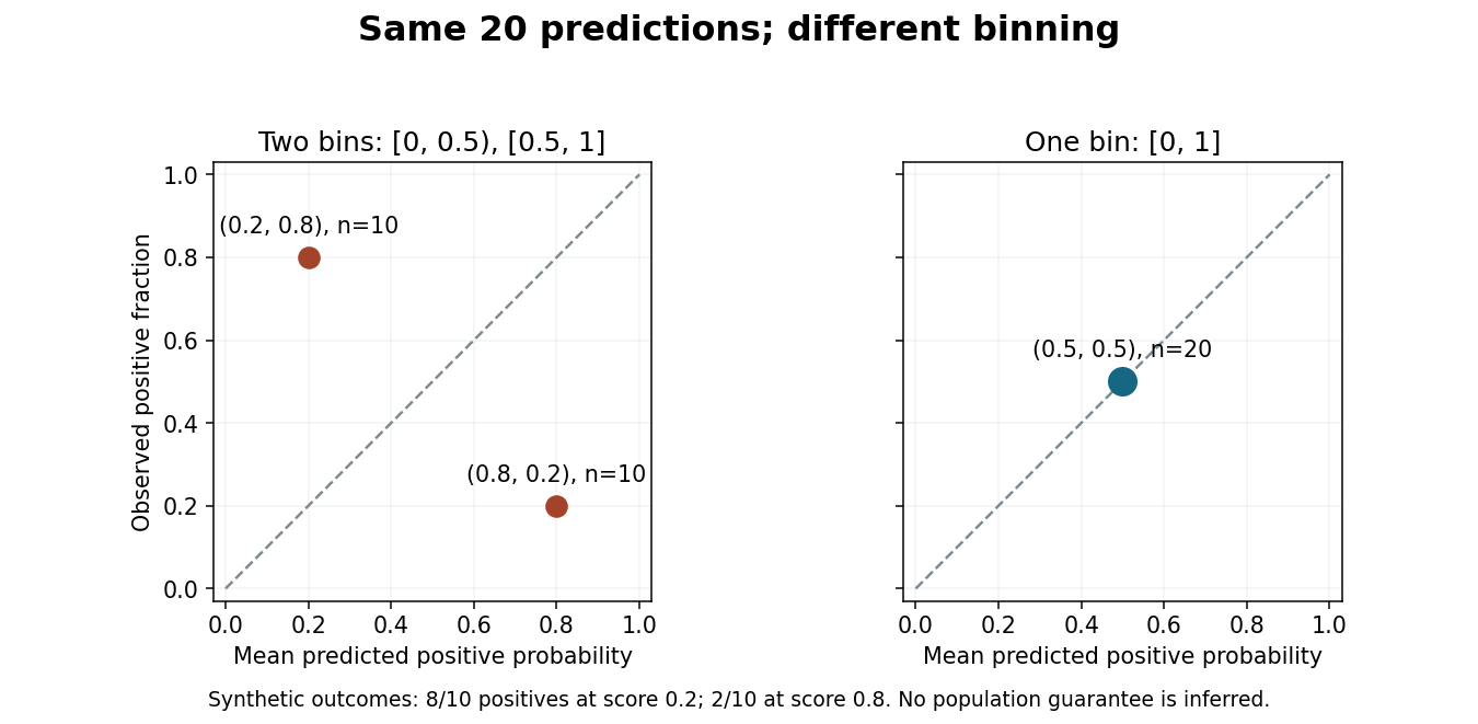
Merging bins can hide disagreement in a reliability diagram.
Original synthetic binary classification example with the same 20 predictions and outcomes in both panels. Points show positive-class frequencies; the diagram does not establish a population guarantee. Details.Report bin definitions and counts, since a point based on ten cases has different sampling uncertainty from one based on thousands. Some classification diagrams instead plot confidence in the selected label against the fraction of correct selections. That convention and the positive-class version answer related but distinct questions, so label the axes and the meaning of the outcome explicitly.[ref]
On Calibration of Modern Neural Networks by Chuan Guo and others. Section 2: selected-label accuracy/confidence convention and limitations of a reliability diagram without bin populations
A confidence score is a numerical output used to express how strongly a system supports a prediction, particularly in statistical classification. Its meaning depends on the system: it may be an estimated probability, a distance from a decision boundary, or another score whose ordering is useful. A number between zero and one does not by itself establish a probability interpretation. Probability calibration concerns whether predicted probabilities agree with observed frequencies.[ref]
Probability calibration in the scikit-learn documentation. §1.16, opening explanation of calibrated classifiers and predict_proba versus decision_function
Consider a synthetic binary statistical classification example. Among independent test cases assigned a positive-class score near , suppose actually belong to that class. Their observed fraction agrees with the average predicted probability. If only belong to the positive class, the same scores overstate the observed positive frequency in this group. A reliability diagram groups predictions by their estimated probability and compares each group's mean prediction with its observed positive fraction. Finite groups have sampling variation, so agreement in one group is evidence to assess with its sample size, rather than a guarantee about each case.[ref]
Probability calibration in the scikit-learn documentation. §1.16.1, Calibration curves: binning, average predicted probabilities and fractions of positives
Ordering and probability calibration answer different questions. For scores in , replacing every score by preserves their order but changes to . Thus an unchanged ranking can accompany very different probability statements. Conversely, a system assigning the overall positive fraction to every case can have useful aggregate probability calibration while failing to distinguish cases.
A confidence score can support a threshold for accepting a prediction or passing it to another process. Select and assess that threshold using examples separate from model fitting and representative of the intended inputs. A threshold does not establish its own error rate; observations on suitable test data supply that evidence. Distinguish a positive-class probability from the score of whichever class was selected: they are different quantities when the selected class changes.
Discriminant analysis constructs statistical rules distinguishing labelled classes from their measured feature values. A common generative approach models the class-conditional probability distribution and applies Bayes' theorem to compare posterior class probabilities. Linear discriminant analysis uses multivariate normal distributions with a shared covariance matrix; allowing a different covariance matrix for each class gives quadratic discriminant analysis.[ref]
Linear and Quadratic Discriminant Analysis in the scikit-learn documentation. §1.2.2, probabilistic model and shared-covariance simplification
For two equally likely one-dimensional classes, suppose and . Their log-likelihood ratio isChoosing the larger posterior therefore selects for , with a tie at one. Different class probabilities move this threshold. Estimating means and covariance from training data supplies a fitted rule, while independent evaluation tests whether its assumptions generalize.
For a binary classifier, the conditional probability of the target condition given a positive classification. If its base rate is , its true-positive probability is , and its false-positive probability is , Bayes' theorem gives . The denominator is positive whenever a positive classification can occur.