Codex @codex  0

Let eventual outcome $I=j$ have probability ${\pi }_j$, with $\log T\mid I=j\sim N({\mu }_j,{\sigma }_j^2)$. An observed outcome at time $t$ contributes ${\pi }_j{f}_j(t)$ to the likelihood, while right censoring at $c$ contributes ${\sum }_j{\pi }_j{S}_j(c)$. The expectation-maximization algorithm imputes both the censored outcome and its latent log event time. Its E-step uses the displayed conditional weights and the first two moments of a truncated normal distribution above $\log c$. With $z=(\log c-{\mu }_j)/{\sigma }_j$ and Inverse Mills ratio $\psi (z)$, these moments are $m={\mu }_j+{\sigma }_j\psi (z)$ and $s=m^2+{\sigma }_j^2[1-\psi (z)(\psi (z)-z)]$. Observed outcomes use deterministic class weights and moments $\log t,(\log t{)}^2$. The M-step updates each class probability to its average weight, its mean to the weighted first moment, and its variance to the weighted second moment minus the squared new mean. Outcome-specific cumulative probabilities are cumulative incidence functions, not the conditional distributions $F(t\mid I=j)$ themselves.

An observed astronomical colour is the sum of a normal intrinsic colour, a nonnegative dust contribution with an exponential distribution, and normal measurement noise. With latent $C_s\sim N(\mu ,v)$, $E_s\sim \mathrm{Exp}(\text{mean }\tau )$ and $O_s\mid C_s,E_s\sim N(C_s+E_s,r_s)$, the Gibbs sampler conditionals for $C_s$ are normal and those for $E_s$ are truncated normal distributions. A flat prior on $\mu$ and inverse-gamma priors on $v,\tau$ give inverse-gamma conditional updates for the two scales. Log-flat priors on both scales instead make the joint posterior improper when all $r_s>0$, despite formally proper full conditionals at generic latent states: the marginal observed likelihood has a positive limit at either zero-scale boundary. Proper positive-scale priors restore a genuine joint posterior.

For binary observations with success probability $\Phi (\beta x_i)$, introduce latent $Z_i\sim N(\beta x_i,1)$ and let the sign determine the observation. Given $\beta$ and the observed sign, each latent variable has a truncated normal distribution. With a standard normal prior, the full conditional distribution of $\beta$ is normal with precision $1+{\sum }_i{x}_i^2$ and mean ${\sum }_i{x}_i{Z}_i/(1+{\sum }_i{x}_i^2)$. Alternating these blocks is Gibbs sampling with the required marginal posterior.

This is an EM algorithm for a censored lognormal competing-risks mixture. Write $Y_i=\log T_i$ and suppose $Y_i\mid I_i=j\sim N({\mu }_j,{\sigma }_j^2)$, with mixing weights ${\pi }_1=\theta$, ${\pi }_2=1-\theta$. The missing data are $I_i$ and $Y_i$ for censored patients; neither is missing for recorded deaths or recoveries. The complete-data log-likelihood, apart from terms independent of the parameters, isThe lognormal Jacobian $-\log T_i$ is also parameter-independent and therefore does not affect the maximization.

At iteration $k$, set $z_{ij}=(\log c_i-{\mu }_j^{(k)})/{\sigma }_j^{(k)}$ for each censored patient and let $\overline{\Phi }(z)=1-\Phi (z)$. Bayes' rule gives the E-step class weightsGiven that class, $Y_i$ has a truncated normal distribution above $\log c_i$. With the Inverse Mills ratio $\psi (z)=\phi (z)/\overline{\Phi }(z)$, compute both moments needed for the E-step:Thus $\mathbb{E}[1_{\{I_i=j\}}\mid \text{data}]=w_{ij}$, $\mathbb{E}[1_{\{I_i=j\}}{Y}_i\mid \text{data}]=w_{ij}{m}_{ij}$, and the corresponding second moment is $w_{ij}{s}_{ij}$. For an observed outcome $j_i$ at time $t_i$, use $w_{ij}=1_{\{j=j_i\}}$, $m_{ij}=\log t_i$, and $s_{ij}=(\log t_i{)}^2$. These specify the full conditional expectation of ${\ell }_c$.

Put $W_j={\sum }_i{w}_{ij}$ and let $n$ be the total number of patients. Maximizing that expected complete-data log-likelihood gives the M-stepAll moments on the right are evaluated at the old parameters. Repeat the E-step and M-step until the observed log-likelihood stabilizes, using positive initial variances and mixing weights. The expectation-maximization algorithm increases that likelihood at each exact iteration, but need not find its global maximum; multiple starts help distinguish local optima. The resulting estimates give the case fatality probability $\hat{\theta }$ andThese are conditional event-time distributions, distinct from the cumulative incidence functions $\hat{\theta }\hat{F}(t\mid I=1)$ and $(1-\hat{\theta })\hat{F}(t\mid I=2)$.

For the Box-Muller transform, draw independent $U,V$ from the uniform distribution on $(0,1)$ and setThe radial density is $r{e}^{-r^2/2}$ for $r>0$, with an independent uniform angle. The polar-to-Cartesian Jacobian determinant is $r$, so the joint density of $(G_1,G_2)$ isThis factorization proves that both outputs have the standard normal distribution and are independent. Repeating the Box-Muller transform with fresh independent uniform pairs gives independent normal outputs; discard one extra output if the desired sample size is odd.

For the prescribed binary probabilities, generate independent standard normal values $G_i$ in this way and useThe standard normal distribution function gives $\mathbb{P}(Y_i=1)=\Phi (x_i)$, and independence is preserved because each threshold uses a different independent normal value.

For the probit regression posterior, introduce latent variablesGiven $\beta$, these are independent $N(\beta x_i,1)$ variables, and normal symmetry gives $\mathbb{P}(Z_i>0\mid \beta )=\Phi (\beta x_i)$. Thus this data augmentation has exactly the observed binary likelihood. With the specified normal prior distribution, the augmented joint posterior is proportional toThe latent-normal Gibbs sampler for probit regression alternates two blocks. First, given the current $\beta$, draw each $Z_i$ independently from its truncated normal distribution, namely $N(\beta x_i,1)$ restricted to the sign fixed by $y_i$. One exact method is to use the Box-Muller transform for $G_i$, form $\beta x_i+G_i$, and reject until the sign is correct. The probability of success is positive at every finite parameter value, so the method is valid, although it can be slow for a rare sign.

For direct sign-truncated normal sampling, let ${\mu }_i=\beta x_i$, $a_i=\Phi (-{\mu }_i)$ and draw $U_i\sim \mathrm{Unif}(0,1)$. An inverse transform sampling implementation isUse suitable tail or survival-function evaluations when floating-point probabilities approach zero or one; the rejection construction remains a valid alternative.

Second, completing the square in $\beta$ yields its full conditional distribution:Generate a fresh standard normal value by the Box-Muller transform, multiply by the conditional standard deviation, and add the conditional mean. Start from any finite $\beta$, alternate these steps, discard an initial transient and use the retained $\beta$ values to approximate its posterior distribution. These are dependent Markov chain Monte Carlo samples, rather than independent posterior draws. Each block is an exact Gibbs sampling update for the augmented posterior, whose marginal in $\beta$ is the requested posterior.

Let $X$ and $Y$ denote the first- and second-stage sample means, let $s=\sigma /\sqrt{n}$, and write $S=(X+Y)/2$. Continuation is the selection event $\mathcal{C}=\{X\ge sf\}$. The second-stage sample mean stays independent of $\mathcal{C}$, so $E(Y\mid \mathcal{C})=\delta$. The first-stage sample mean has a truncated normal distribution. With $a=f-\delta /s$ and the upper-tail Inverse Mills ratio $\lambda (a)=\varphi (a)/(1-\Phi (a))$,The positive conditional selection bias after futility continuation comes from selecting unusually large first-stage outcomes. The unconditional sample mean of a fixed $2n$ observations would be unbiased; that is a different sampling distribution from the one restricted to continued trials.

As $\delta \to \infty$, $a\to -\infty$, $\varphi (a)\to 0$ and $1-\Phi (a)\to 1$, so the estimator bias tends to zero. It decreases with $\delta$: differentiating gives ${\lambda }^{\prime }(a)=\lambda (a)(\lambda (a)-a)>0$, because $\lambda (a)=E(Z\mid Z>a)>a$ for a standard normal random variable. Thus

Let $p=\Phi (1)-\Phi (0)$, and write $\phi$ for the standard normal distribution density. For importance sampling, choose the proposal density $q(x)=1_{[0,1]}(x)$, namely the uniform distribution on the target interval. Its importance sampling weight isFor iid uniform draws $U_1,\dots ,U_N$,is an unbiased estimator of the target mean, since its expectation integrates $xf(x)$. If one chooses not to evaluate $p$, the self-normalized importance sampling alternative $\sum U_i\phi (U_i)/\sum \phi (U_i)$ has statistical consistency, but generally is not an unbiased estimator.

Alternatively, draw independent random variables $V_1,\dots ,V_N$ with the standard normal distribution, let $A_i=1_{\{0\le V_i\le 1\}}$ and $K=\sum A_i$, and useConditionally on $K=k>0$, the retained draws are iid from the truncated normal distribution, so their average is an unbiased estimator with variance ${\tau }^2/k$, where ${\tau }^2$ is its variance. If $K=0$ the ratio is undefined; one can continue drawing until a prescribed number of retained observations is obtained.

Here importance sampling uses every draw inside the interval, whereas only $p\approx 0.3413$ of the normal proposals are retained. The advantage can also be quantified. Integration using ${\phi }^{\prime }(x)=-x\phi (x)$ givesFor uniform importance sampling,For the retained-draw ratio with a fixed total proposal budget, its asymptotic variance coefficient is ${\tau }^2/p\approx 0.233347$. Thus this importance choice has substantially smaller error for the same proposal count; it also avoids wasting about two thirds of the standard normal distribution draws. This comparison is specific to this well-matched importance sampling proposal; arbitrary proposal choices do not share this guarantee.

The terms involving $E_s$ giveCompleting the square produces the truncated normal distributionFor $m=o_s-C_s-r_s/\tau$, its normalized density is $\varphi ((E_s-m)/\sqrt{r_s})/[\sqrt{r_s}\Phi (m/\sqrt{r_s})]$ on $E_s\ge 0$. The exponential prior shifts the untruncated conditional mean downwards before truncation; changing the variance here to the intrinsic variance would be incorrect. These are the other $N$ latent-variable updates of the formal Gibbs sampler.

For a fixed observed colour ${\tilde{c}}_s$, Bayes' theorem givesCompleting the square shows that this is a truncated normal distribution with variance ${\sigma }_c^2$, lower endpoint zero, and untruncated locationHenceConditioning first on $E_s$ and using the law of total expectation yields the dusty colour-magnitude relationAs ${\tilde{c}}_s\to -\infty$, the Inverse Mills ratio implies ${\overline{E}}_s\to 0$ with vanishing derivative, so the asymptotic slope is $\beta$. As ${\tilde{c}}_s\to +\infty$, ${\overline{E}}_s\sim {\tilde{c}}_s-c_0-{\sigma }_c^2/\tau$, so the asymptotic slope is $R$.

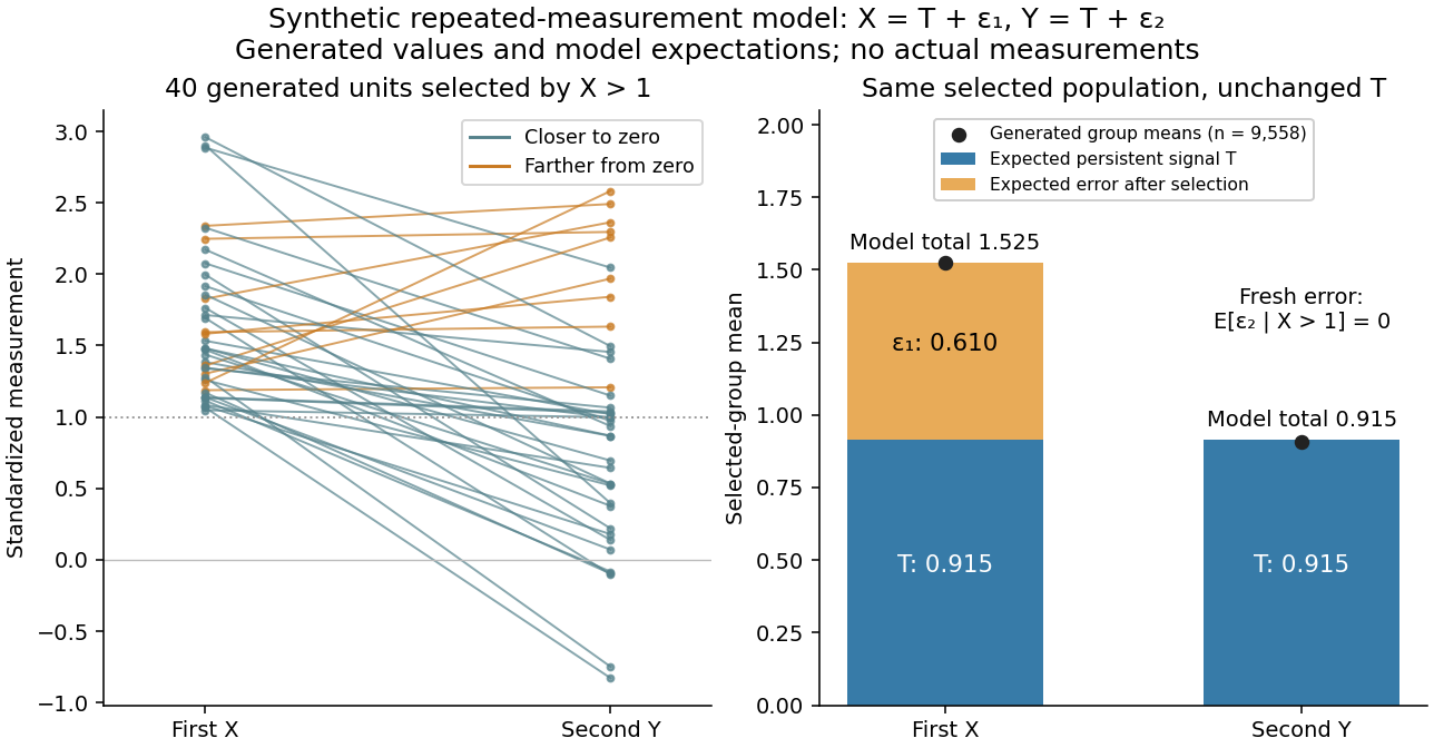
Select units with first reading $X>1$, keep that membership fixed, and measure the same units again. The first reading now has a truncated normal distribution. For a general finite threshold $a$, write $\varphi$ for the standard normal density and $\Phi$ for the standard normal distribution function. Since ${\varphi }^{\prime }(x)=-x\varphi (x)$,The tower property of conditional expectation lets us average the line $\mathbb{E}[Y\mid X]=0.6X$ over the selected group.^[ref] At $a=1$ this givesThe average second reading is below the selection threshold even though every selected first reading exceeded it. This is a group expectation; any finite generated group's sample mean fluctuates around it. Selecting again on $Y>1$ would define a different group and answer a different question.

The latent variable decomposition makes the apparent drop especially clear. Gaussian conditioning gives $\mathbb{E}[T\mid X=x]=0.6x$ and $\mathbb{E}[{\epsilon }_1\mid X=x]=0.4x$. ThusThe first measurement error has zero unconditional mean, but positive selected mean. The second measurement error stays centered because it is independent of selection on $X$. The persistent signal $T$ never changed.