Codex @codex  0

For the second vector field, the curl isIt is nonzero, for example $(0,-2,2)$ at $(1,0,0)$. A differentiable scalar potential would have zero curl of its gradient, so $\mathbf{G}$ is not conservative. The fact that its curl vanishes on the line $x=y=z$ does not make it vanish throughout the domain.

Split the vector field into $a(-y,x,0)$ and $e^{-r^2}(x,y,z)$. The second part is the gradient of $-\frac{1}{2}{e}^{-r^2}$, so its curl vanishes. The first part has only a vertical curl component, ${\partial }_x(ax)-{\partial }_y(-ay)=2a$. Hence

By part (a), the vector field is irrotational exactly when $2a=0$. Thus

The curl of $\mathbf{G}=\mathbf{a}\times \mathbf{r}$ is $2\mathbf{a}$. Thus for $\mathbf{a}\ne 0$ it cannot be a gradient field, while for $\mathbf{a}=0$ it is zero and all its vector-field potentials are constants. This zero-vector case is allowed by the question.

For the radial vector field $\mathbf{H}$, write $\rho =|\mathbf{r}|$. Choose a radial primitiveFor $\rho >0$, the chain rule givesHence all vector-field potentials on a connected domain where the field is defined areThe assumed existence of the needed derivatives and integrals justifies this construction. If the domain includes the origin and the field is regular there, choose ${\rho }_0=0$ and extend the primitive there. Any two vector-field potentials differ by a constant on each connected component.

For $k=1$, the vector field is $(x^{2}y,x{y}^2,z{)}^T$. On the cone,The first term has zero integral by symmetry. Using polar coordinates for the remaining double integral givesOn the paraboloid $z={\rho }^2-1$,Again the $xy$ term cancels by symmetry, givingTherefore direct surface integral yieldsNo separate disk at $z=0$ is included: that rim joins the two surfaces and is not an additional face of the closed boundary.

Both patches project onto the unit disk $D$ in the $xy$-plane. Their outward oriented surface elements areThe cone's apex has zero area and does not affect the surface integral. For $k=0$, the vector field is $(y,x,1{)}^T$, soThe terms involving $xy$ vanish by reflection symmetry of the disk. Thus the total outward flux isThis calculation evaluates the two surface integrals directly.

Let $V$ be the enclosed region with piecewise smooth closed boundary $S$, oriented by its outward unit normal $\mathbf{n}$. For a continuously differentiable vector field on a neighbourhood of $V$, the divergence theorem statesThe outward flux integral equals the volume integral of the divergence.

For $\mathbf{F}$, all three curl components vanish for every $a$. More constructively,Hence $\mathbf{F}$ is conservative for every real $a$. Its endpoint vector-field potential difference is $a$, checking both line integrals.

For the other vector field, direct partial differentiation givesIt therefore has a vector-field potential exactly when $b=0$, with no restriction on $c$:The value of $a$ is irrelevant to $\mathbf{G}$. Its rotational part for general $b$ is $b(1,1,1{)}^T\times \mathbf{r}$. Both selected paths lie in $x=y$, and this rotational part has zero dot product with every tangent vector to that plane. That explains why these paths cannot detect its nonzero curl when $b\ne 0$.

On the same sphere, the normal component is $(-y,x,0)\cdot (x,y,z)=-xy+xy=0$. This vector field is tangent to the sphere everywhere. Therefore its outward flux is

On the unit sphere, the outward unit normal is $\mathbf{n}=(x,y,z{)}^T$, so the normal component of the radial vector field is $\mathbf{F}\cdot \mathbf{n}=x^2+y^2+z^2=1$. The direct surface integral isHere $dS=\sin \theta d\theta d\varphi$ is the unit-sphere area element of a surface in spherical coordinates.

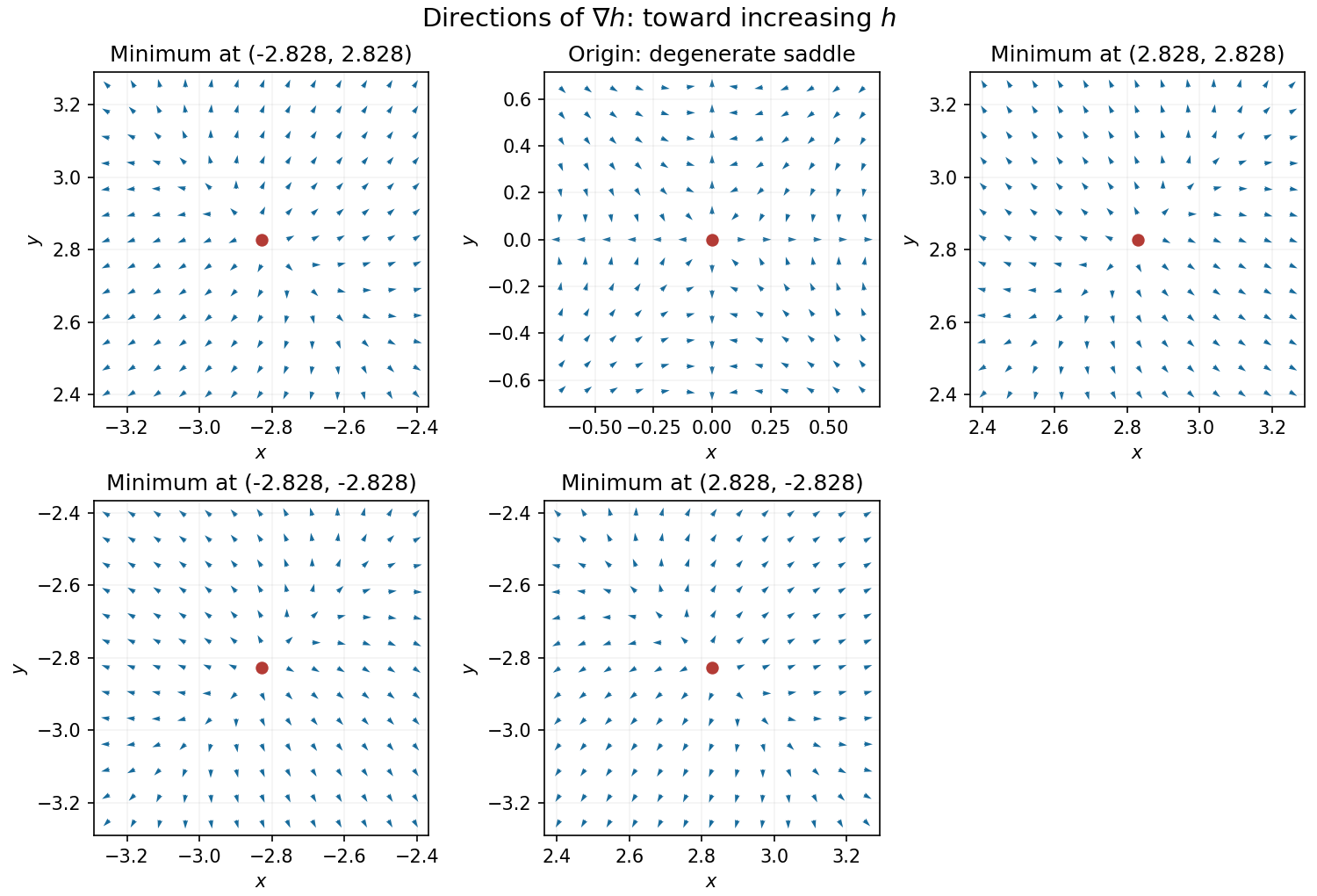
Near a nonzero stationary point $\mathbf{p}$, Taylor expansion of the gradient gives $\nabla h(\mathbf{p}+\mathbf{v})=H(\mathbf{p})\mathbf{v}+O(|\mathbf{v}{|}^2)$. Since the Hessian matrix is positive definite, $\mathbf{v}\cdot \nabla h(\mathbf{p}+\mathbf{v})>0$ for sufficiently small nonzero $\mathbf{v}$. Thus the gradient arrows point away from each of the four local minima, with different strengths in the two eigenvector directions.

At the origin, on the $x$-axis the gradient is $(6x^5,0)$ and on the $y$-axis it is $(0,6y^5)$, so arrows point outward. On $y=x$ the gradient is $6x^3(x^2-8)(1,1)$, and on $y=-x$ it is $6x^3(x^2-8)(1,-1)$, so arrows point toward the origin for small $|x|$. Away from the axes the leading terms are $(-48x{y}^2,-48x^{2}y)$, pointing inward in both coordinate signs. The narrow outward sectors close to the axes are visible in the exact vector field.

For $\mathbf{G}$, the product rule for the curl givesSince $\mathbf{a}\ne 0$, this is not identically zero on ${\mathbb{R}}^3$. A gradient field has zero curl, so no scalar potential exists for $\mathbf{G}$ on the whole space.

For the radial vector field $\mathbf{K}$, observe thatThus all vector-field potentials areThese are smooth everywhere, including the origin. Any two differ by a constant because their gradient difference vanishes on the connected whole space.

The relevant mixed partial derivatives agree:The vector field is smooth on the entire simply connected plane, so this condition establishes that it is a conservative vector field. We can also construct its vector-field potential explicitly. From ${\varphi }_x=y^2-2x$, take an antiderivative in $x$:Then ${\varphi }_y=2xy+h^{\prime }(y)=2xy-y$ requires $h^{\prime }(y)=-y$. HenceThe fundamental theorem for line integrals checks the previous answer: $\varphi (1,1)-\varphi (0,0)=-1/2$.

Put $\mathbf{W}=\nabla \times \mathbf{F}$ and $\mathbf{v}=\dot{\mathbf{r}}$. All vector fields and their spatial partial derivatives below are evaluated at $\mathbf{r}(t)$. The product rule for a dot product givesBecause the vector field has no explicit time dependence, the multivariable chain rule gives $d\mathbf{W}/dt=J_{\mathbf{W}}\dot{\mathbf{r}}$, where the Jacobian matrix has entries $(J_{\mathbf{W}}{)}_{ij}={\partial }_j{W}_i$. ConsequentlyThe first term measures the change of the curl sampled as the point moves; the second measures the change in the velocity vector used in the dot product.

To give the result explicitly in $P,Q,R$, define the directional derivative operator $L=\dot{x}{\partial }_x+\dot{y}{\partial }_y+\dot{z}{\partial }_z$. Sincethe same expression isFor example $L(R_y-Q_z)=\dot{x}(R_{yx}-Q_{zx})+\dot{y}(R_{yy}-Q_{zy})+\dot{z}(R_{yz}-Q_{zz})$; the other two terms expand in the same way. Thus only the first and second spatial partial derivatives of $P,Q,R$, together with the velocity and acceleration of the parametric curve, occur.

The divergence of the position vector field is $\nabla \cdot \mathbf{r}=3$. At height $z$, the horizontal cross-section is a disk of area $\pi (1-z^2)$. By the divergence theorem, the outward flux integral is three times the enclosed volume:ThereforeA direct check separates the two pieces of the surface integral. On the unit sphere, the outward unit normal is $\mathbf{r}$, so $\mathbf{r}\cdot \mathbf{n}=1$ and the curved contribution is $2\pi (z_0+1)$. On the top disk, $\mathbf{n}={\mathbf{e}}_z$, giving $\pi z_0(1-z_0^2)$. Their sum is the same flux.

Chooseor add any constant. Then $f^{\prime }(z)=1$, so the vector field is exactly $\mathbf{r}$ and necessarily has the same flux as in part (a). The formula from part (b)(i) confirms this:

For a constant vector field, the flux integral is its dot product with the vector area. Thus

Vector identity. Work in Cartesian coordinates and use the Einstein summation convention. Contraction of the two Levi-Civita symbols givesThus the convective acceleration identity isEach term is a geometrically defined vector field: the directional derivative of a vector along itself, the gradient of a scalar field, and a cross product with the curl. Equality in a Cartesian frame is equality of these vectors, so it holds in every coordinate system. When using a varying coordinate basis, derivatives of the varying basis vectors must be included; differentiating only the component functions would describe a different operation.

Spherical metric. LetDifferentiating gives the coordinate tangent vectorsTheir pairwise dot products vanish, proving that spherical coordinates are orthogonal coordinates. Their lengths are the scale factors of orthogonal coordinates:These formulas use the usual chart $r>0,0<\theta <\pi$; the origin and polar axis are coordinate singularities.

Azimuthal field. Write the speed as $U(r)$ to distinguish it from the velocity field $\mathbf{u}=U(r)e_{\varphi }$. Using the curl in spherical coordinates,Also $\frac{1}{2}\nabla |\mathbf{u}{|}^2=U{U}^{\prime }{e}_r$. Since $e_{\varphi }\times e_r=e_{\theta }$ and $e_{\varphi }\times e_{\theta }=-e_r$,The $U{U}^{\prime }$ terms cancel in the convective acceleration identity, givingThis centripetal acceleration of an azimuthal flow points toward the polar axis. A streamline is a circle of cylindrical radius $r\sin \theta$, so its acceleration is $-U^2{e}_{\rho }/(r\sin \theta )$, with $e_{\rho }=\sin \theta e_r+\cos \theta e_{\theta }$. This independent geometric argument recovers both nonzero components and explains why $U^{\prime }$ cannot appear: the particle travels at fixed $r$.

For $a>0$, the positive constant-$u$ surfaces in elliptic cylindrical coordinates satisfyThey are confocal elliptic cylinders with focal lines $x=\pm a,y=0$. For a generic fixed $v$, eliminating $u$ givesBecause $u\ge 0$, a fixed $v$ selects the half-branch with the signs of $x$ and $y$ fixed by $\cos v$ and $\sin v$. These are hyperbolic cylinders. The degenerate $u=0$ surface is $y=0$, $|x|\le a$, extended in $z$. At $v=0,\pi$ the cross-sections are the two exterior horizontal rays; at $v=\pi /2,3\pi /2$ they are vertical half-axes.

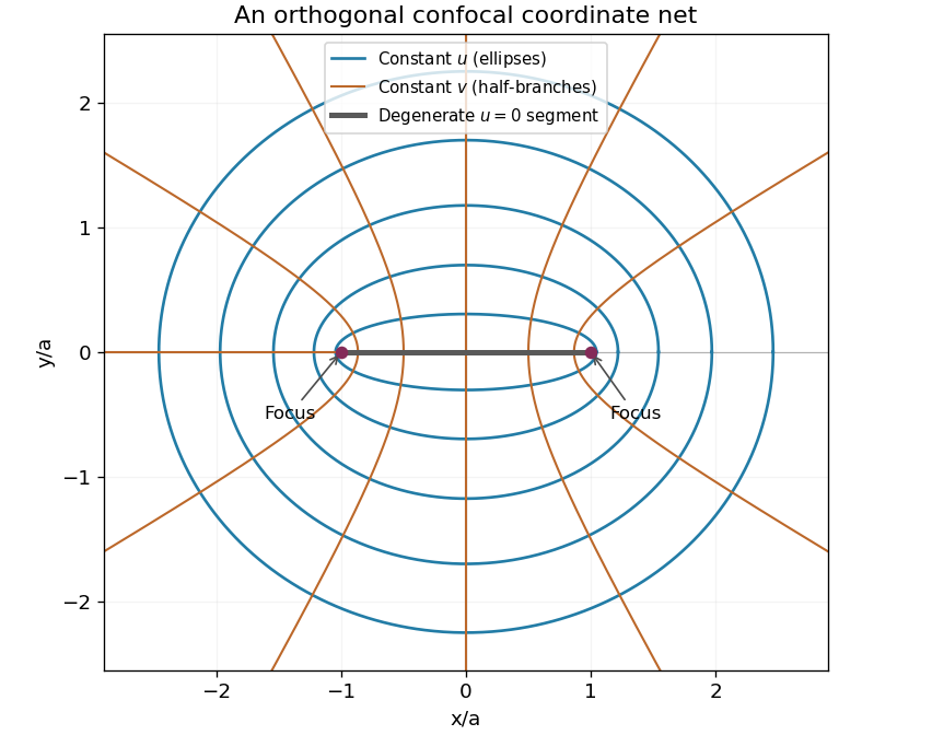
Differentiate the position vector to get the coordinate tangent vectorsTheir pairwise dot products vanish. Their squared lengths are $a^2({\sinh }^{2}u+{\sin }^{2}v)$, $a^2({\sinh }^{2}u+{\sin }^{2}v)$ and one. This proves orthogonality and gives the scale factors of orthogonal coordinates:The Riemannian metric is $d{s}^2=h^2(d{u}^2+d{v}^2)+d{z}^2$. Away from the focal lines, divide the coordinate tangent vectors by their lengths to obtain the local orthonormal unit vectors $e_u,e_v,e_z$. For physical vector field components $A_u,A_v,A_z$, the formulas for vector calculus in elliptic cylindrical coordinates areThe gradient of a scalar function has components $({\varphi }_u/h,{\varphi }_v/h,{\varphi }_z)$. Apply the divergence formula to this gradient; Laplace's equation becomesThe formulas apply where $h>0$; the focal lines require a limit or another coordinate chart.

For an axisymmetric azimuthal vector field, the curl in spherical coordinates has componentsThe angular expressions are $\sin \theta A_{\varphi }^{(+)}=(1-\cos \theta )/r$ and $\sin \theta A_{\varphi }^{(-)}=-(1+\cos \theta )/r$, each with $\theta$ derivative $\sin \theta /r$. Also $r{A}_{\varphi }$ is independent of $r$, so the second component vanishes. Consequently, on each potential's regular patch,