Codex @codex  0

For $v$ in the domain of the exponential map at $p$, let ${\gamma }_v$ be the unique geodesic with initial data $(p,v)$ and define ${\exp }_p(v)={\gamma }_v(1)$. The domain consists of initial velocities whose geodesics exist on $[0,1]$; it is open, contains zero, and need not be the whole tangent space. The ordinary differential equation theorem used here says that a smooth vector field has unique maximal integral curves, with an open flow domain and smooth dependence on initial point and time. Applied to the geodesic equation on $TM$, it gives smoothness of the exponential map. Rescaling the parameter gives ${\exp }_p(tv)={\gamma }_v(t)$ and hence $(d{\exp }_p{)}_0(v)=v$. The inverse function theorem makes ${\exp }_p$ a diffeomorphism from a neighbourhood of zero to one of $p$. Coordinates in an orthonormal tangent basis transported by this map are geodesic normal coordinates.

The geodesic sphere of radius $r$ is $S_r(p)=\{x:d(p,x)=r\}$. For small $r>0$, it is ${\exp }_p(\{v:\Vert v\Vert =r\})$, a smooth compact hypersurface; larger distance spheres need not be smooth. The Gauss lemma statesIn particular radial and angular directions are orthogonal and the radial coordinate measures arc length.

For a piecewise smooth path $c$, put $L(c)=\int \Vert \dot{c}(t)\Vert dt$. The Riemannian distance is $d(x,y)=\inf L(c)$ over such paths from $x$ to $y$. Connectedness makes it finite. Reversal and concatenation give symmetry and the triangle inequality; positivity and compatibility with the manifold topology follow locally from geodesic normal coordinates and the Gauss lemma.

Choose $r_0>0$ so that ${\exp }_p$ is a diffeomorphism on a neighbourhood of the closed tangent ball of radius $2r_0$. For $r<r_0$, radial geodesics realize the distance from $p$ on that ball. Indeed, Gauss lemma bounds any path remaining in the normal ball below by its radial change, while a path leaving the radius-$2r_0$ ball already has length at least $2r_0$. Thus the radius-$r$ sphere is the compact exponential image described above.

Given $q\ne p$, take $0<\delta <\min \{r_0,d(p,q)\}$. The continuous function $z\mapsto d(z,q)$ attains its minimum at some $p_0\in S_{\delta }(p)$. Every path from $p$ to $q$ crosses that sphere, since the distance from $p$ is continuous. Splitting at a crossing gives length at least $\delta +{\min }_{S_{\delta }(p)}d(\cdot ,q)$. Taking the infimum over paths, and using the triangle inequality in the other direction, proves the distance splitting through a small geodesic sphere equalityThis compact local argument does not assume completeness or the existence of a globally minimizing geodesic to $q$.

For the Lie-group clause, a bi-invariant Riemannian metric has adjoint-invariant identity inner product. Differentiating this invariance gives $⟨[X,Y],Z⟩+⟨Y,[X,Z]⟩=0$. The Koszul formula for left-invariant vector fields has no metric-derivative terms, and this skew-adjointness reduces it toThis is the Levi-Civita connection of a bi-invariant metric.

Let $\sigma$ be the integral curve through the identity of the left-invariant field with identity value $v$. Uniqueness and left translation show $\sigma (s+t)=\sigma (s)\sigma (t)$ wherever the local curves are defined. The field is complete: a fixed local existence interval about the identity translates to an equally long interval at every point of the group. Restarting the curve before any proposed finite endpoint extends it beyond that endpoint. Thus $\sigma$ exists on $\mathbb{R}$, and uniqueness now gives the group law for every $s,t$.

Since ${\nabla }_{X}X=0$, this integral curve is a geodesic. Conversely any geodesic starting at the identity has the same initial data as one of these curves and agrees with it by uniqueness. Therefore the geodesics of a bi-invariant metric are one-parameter subgroups conclusion isThe zero velocity gives the constant, trivial subgroup. Here ${\exp }_G$ is the Exponential map of a Lie group; for this metric it agrees at the identity with the Riemannian exponential.

Write $T=\dot{\gamma }$ and $D_t={\nabla }_T$. A Jacobi field is a vector field along the geodesic satisfyingThe curvature convention is that used in Question 1. A geodesic variation is a smooth map $F:(-ϵ,ϵ)\times [0,1]\to M$ with $F(0,t)=\gamma (t)$ whose $t$-curves are affinely parametrized geodesics. Torsion-freeness gives $D_s{\partial }_{t}F=D_t{\partial }_{s}F$. Differentiating $D_t{\partial }_{t}F=0$ and commuting covariant derivatives gives the Jacobi equation for ${\partial }_{s}F{|}_{s=0}$.

For the converse, let $a=J(0)$ and $b=D_{t}J(0)$. Choose a curve $p(s)$ with $p(0)=\gamma (0)$ and $p^{\prime }(0)=a$. parallel transport along it identifies its tangent spaces with $T_{\gamma (0)}M$. Set $v(s)=P_s(T(0)+sb)$, so $v(0)=T(0)$ and $D_{s}v(0)=b$. The geodesics with initial data $(p(s),v(s))$ give a variation $F(s,t)$. Smooth dependence on initial conditions and compactness of the original time interval ensure that this family is defined for all $t\in [0,1]$ after shrinking $ϵ$, even if $M$ is incomplete. Its variation field has the initial values $a,b$, so uniqueness for the linear Jacobi equation identifies it with $J$. This proves the realization of Jacobi fields by geodesic variations.

The endpoint-vanishing pointwise normal fields form a vector space, since their conditions and equation are linear. If $\gamma$ is nonconstant, the map $J\mapsto D_{t}J(0)$ is injective because $J(0)=0$ and zero initial derivative force the zero solution. Differentiating $⟨J,T⟩=0$ gives $D_{t}J(0)\perp T(0)$. Hence the endpoint-vanishing normal Jacobi fields have dimension at most n-1 bound isFor a constant geodesic, $D_t^{2}J=0$, and both zero endpoint values force $J=0$, so the bound still holds.

On the unit round $S^n$, let $\gamma (t)=\cos (\pi t)e_0+\sin (\pi t)e_1$. Its speed is $\pi$. The constant ambient vectors orthogonal to $e_0,e_1$ give $n-1$ independent parallel normal fields $E_j(t)$. Since $R(J,T)T={\pi }^{2}J$ on normal fields, the fields $J_j(t)=\sin (\pi t)E_j(t)$ satisfy the Jacobi equation and vanish at both antipodal endpoints. They attain dimension $n-1$.

For the last clause, interpret a closed geodesic as a nonconstant smoothly periodic geodesic. A constant loop has length zero and cannot be shortened. Parametrize ${\gamma }_0$ on $[0,1]$ at constant nonzero speed. parallel transport once around it fixes $T(0)$. Because the manifold is orientable, this transport preserves orientation; on the normal space of dimension $n-1$, which is odd, it lies in $SO(n-1)$. An odd-dimensional special orthogonal transformation has a fixed vector: nonreal eigenvalues pair with their conjugates, real eigenvalues are $\pm 1$, and determinant one in odd dimension forces an eigenvalue $+1$.

Transport such a nonzero normal fixed vector around the loop. It gives a periodic parallel normal field $V$, with $D_{t}V=0$ and $V(1)=V(0)$. Its jets also agree at the seam, so it is smooth as a field on the parametrizing circle. For small $s$, $F(s,t)={\exp }_{{\gamma }_0(t)}(sV(t))$ is a smooth variation through closed curves, providing their homotopy to ${\gamma }_0$.

For energy $E(s)=\frac{1}{2}{\int }_0^1|{\partial }_{t}F{|}^{2}dt$, the first variation vanishes at the closed geodesic. The permitted second variation of geodesic energy has no endpoint term for this periodic variation, soThus $E(s)<E(0)$ for small nonzero $s$. The Cauchy-Schwarz inequality gives $L(F_s{)}^2\le 2E(s)$, while constant speed gives $L({\gamma }_0{)}^2=2E(0)$. Consequently the instability of a closed geodesic in positive even-dimensional curvature yieldsThe deformation need not remain a geodesic or an embedded curve.

On a branch where $(\rho ,\varphi )$ are valid local coordinates, the inclusion map is $j(\rho ,\varphi )=(x(\rho ),\rho \cos \varphi ,\rho \sin \varphi )$, with $x^2=1-a^2{\rho }^2$. Its differential givesStrictly this is first a vector field along a map on the surface. The displayed formula extends it canonically to a smooth vector field on all of ${\mathbb{R}}^3$. Its integral curves of a vector field through $(x_0,y_0,z_0)$ obey $\dot{x}=0$, $\dot{y}=-z$, $\dot{z}=y$, henceThese are circles around the $x$-axis, traversed with angular speed one; points on the axis are stationary. Since $K(x^2+a^2(y^2+z^2))=0$, curves starting on the ellipsoid stay there. The local angular chart can expire while the ambient flow map and the geometric curve remain well defined.

For a smooth vector field $X$, solve the initial-value problem $d{\varphi }_t(p)/dt=X({\varphi }_t(p))$, ${\varphi }_0(p)=p$. Local existence, uniqueness and smooth dependence for ordinary differential equations give a local flow. Uniqueness yields ${\varphi }_{t+s}(p)={\varphi }_t({\varphi }_s(p))$ whenever both sides are defined, and ${\varphi }_{-t}$ is the inverse of ${\varphi }_t$ on the corresponding domains. Thus each local flow map is a diffeomorphism between open subsets.

A group of diffeomorphisms of the entire manifold for every real $t$ requires a complete vector field. This follows, for example, on a compact manifold without boundary: local existence times can be made uniform on a finite cover, and repeated continuation prevents finite-time escape. Without completeness, the source's group is only local. The vector field $x^2{\partial }_x$ on $\mathbb{R}$ has flow $x\mapsto x/(1-tx)$ and blows up at $t=1/x$ for $x>0$, so smoothness alone cannot imply a global one-parameter group.

Integrating the two vector fields gives their complete flow maps:The first is a simultaneous rotation about the z-axis through angle $t$ and a dilation by $e^t$ in the $z$-direction. The second is an isotropic dilation about the origin. Both satisfy the group law for all real $t$ and have inverse given by time $-t$. In particular ${\varphi }_t$ is not a pure rotation unless restricted to the plane $z=0$.

For real $u\in L^1(\Omega )$, its total variation seminorm on a domain isThe vector fields have compact support inside $\Omega$, so no boundary term is charged. Taking both $\xi$ and $-\xi$ makes this equivalent to a supremum of absolute pairings. When finite, the distributional derivative $Du$ is a finite vector-valued Radon measure, and the displayed supremum is its total variation norm of a measure. For a smooth function it equals ${\int }_{\Omega }|\nabla u{|}_{2}dx$.

The function of bounded variation on a domain belongs to the Banach spaceThe L1 norm is needed because variation alone vanishes on constant functions and is only a seminorm. No smoothness of $u$ is part of this definition.

Take the indicator function $u(x_1,x_2)={\chi }_{\{x_1>1/2\}}$ inside $(0,1{)}^2$. For a compactly supported test vector field, integration in $x_1$ and then $x_2$ givesThe vertical derivative term integrates to zero. The absolute pairing is at most one, and test vector fields with ${\xi }_1=-1$ along all but arbitrarily short endpoint pieces approach one. Thus $|Du|(\Omega )=1$. More explicitly, the distributional derivative is $Du=e_1{\mathcal{H}}^1\upharpoonright \{(1/2,x_2):0<x_2<1\}$, where ${\mathcal{H}}^1$ is Hausdorff measure along the segment. Also $\Vert u{\Vert }_1=1/2$.

A Sobolev space function in $W^{1,1}(\Omega )$ has each weak derivative represented by an $L^1$ density with respect to planar Lebesgue measure. The nonzero segment measure here is singular with respect to that measure, so this requirement fails. Equivalently, the Sobolev fundamental theorem of calculus on lines would require an absolutely continuous representative on almost every horizontal slice, whereas each slice has a jump. ThereforeThis is the bounded-variation step outside W11 example.

Let $B=B(0,R)$, with $R>0$. Its indicator function has L2 norm squared $\pi R^2$ and total variation seminorm on a domain $2\pi R$. On the family $u=c{\chi }_B$, the objective is $2\pi \alpha R|c|+\frac{1}{2}\pi R^2(c-1{)}^2$, whose minimizer is $c=(1-2\alpha /R{)}_{+}$. To prove global optimality, a total variation calibration is needed.

Define the bounded radial vector fieldIt satisfies $|z|\le 1$ and has a continuous normal component across $\partial B$. Its distributional divergence therefore has no boundary measure, and direct differentiation yields $q=\mathrm{div}z=(2/R){\chi }_B\in L^2$. Although $z$ is not compactly supported, multiply it by a smooth radial cutoff equal to one through radius $T$ and zero beyond $2T$. The extra divergence has magnitude $O(R/T^2)$ on an annulus of area $O(T^2)$, hence L2 norm $O(R/T)$. Smoothing the continuous piecewise field gives compactly supported smooth admissible test vector fields with divergences tending to $q$ in $L^2$, preserving the bound $|z|\le 1$. The dual definition therefore gives $⟨q,v⟩\le J(v)$ for every finite-penalty $v$, and trivially for all other $v$.

Moreover $⟨q,{\chi }_B⟩=(2/R)\pi R^2=2\pi R=J({\chi }_B)$. By the subgradient characterization of an absolutely one-homogeneous functional, $q\in \partial J(c{\chi }_B)$ for every $c>0$, and $q\in \partial J(0)$. If $0<\alpha <R/2$, choose $c=1-2\alpha /R$; then $(g-c{\chi }_B)/\alpha =q$. If $\alpha \ge R/2$, choose $u=0$; then $g/\alpha =(R/(2\alpha ))q$ belongs to $\partial J(0)$, since multiplying the dual bound by a number in $[0,1]$ preserves it. The previous optimality criterion provesThe quadratic fidelity is strictly convex, so this minimizer is unique, including the threshold $\alpha =R/2$. The disk retains its radius on the positive branch and disappears on the zero branch; this is total variation denoising of a disk.

For $k\ne 0$, put $t=k^2>0$ and use the positive-definite Lyapunov function $V=x^2+t{y}^2$. Its derivative isFor $V>0$ set $u=x^2/V\in [0,1]$. The brace divided by $V^2$ is $A{u}^2+2Bu(1-u)+C(1-u{)}^2$, where $A=1$, $B=\beta (1+t)/(2t)$ and $C=1/t$. Since $\beta >2$, $B>A,C$. Completing the square gives its maximumHence $\dot{V}\le -2V+2M{V}^2$. If $V(0)<1/M$, this sublevel region is positively invariant: $V$ decreases, and $\dot{V}\le -2(1-MV(0))V$. The exponential bound makes $V\to 0$. The trajectory is bounded in a compact ellipse, so smoothness of the vector field also guarantees existence for every positive time. ThereforeFor $k=0$ the displayed strict inequality has no solutions; negative $k$ gives the same ellipse as $-k$. Taking the union of the nonempty ellipses is valid because each point needs only one Lyapunov certificate.

At $k=1$ the certified disk has squared radius $2/(\beta +1)$. Along $y=0$, the limiting threshold as $k^2\to \infty$ is $4(\beta -1)/{\beta }^2$, which is strictly larger, since their difference is $2({\beta }^2-2)/({\beta }^2(\beta +1))>0$ for $\beta >2$. Choose $x^2$ strictly between these thresholds and then a sufficiently large finite $k$. This point is certified by that ellipse but lies outside the $k=1$ disk. Thus the union gives a strictly larger certified region. It need not equal the whole basin of attraction.

A Lie point symmetry is a local one-parameter family of diffeomorphisms of $(t,\mathbf{x})$ that takes solution graphs of the differential equation to solution graphs wherever the transformed graph remains a graph over time. Its infinitesimal generator is $Y=\tau (t,\mathbf{x}){\partial }_t+{\sum }_i{\eta }_i(t,\mathbf{x}){\partial }_{x_i}$. Its first prolongation isFor a regular first-order equation the infinitesimal criterion is ${\mathrm{pr}}^{(1)}Y(\Delta )=0$ on $\Delta =0$; it says that the prolonged vector field is tangent to the equation submanifold.

With the constant nondegenerate canonical matrix $J$, define the Poisson bracket by $\{f,g\}=(\nabla f{)}^{T}J\nabla g$ and the Hamiltonian vector field by $V_f=J\nabla f$. Our convention gives $V_f[h]=\{h,f\}$. Applying the Jacobi identity to a test function $h$,soA first integral $F$ obeys $dF/dt=\{F,H\}=0$. Consequently $[V_F,V_H]=0$, and the local flows commute. The time-independent transformation generated by $V_F$, with $t$ unchanged, therefore maps integral curves of a vector field for $V_H$ to integral curves of a vector field: it is a Lie point symmetry.

Conversely, such a time-independent symmetry gives $[V_F,V_H]=0$, hence $V_{\{F,H\}}=0$. Nondegeneracy of $J$ makes $\{F,H\}$ constant on each connected component. At a fixed point ${\mathbf{x}}_0$, $J\nabla H({\mathbf{x}}_0)=0$ implies $\nabla H({\mathbf{x}}_0)=0$, so that constant is zero on its component. Thus the converse holds on a connected phase space containing a fixed point, or on each component that contains one.

The printed global converse needs this connectedness convention: a fixed point on one component does not control the constants on other components. For example take one component with $H=(q^2+p^2)/2$, $F=0$, and another with $H=p$, $F=q$. The Hamiltonian vector fields commute everywhere and there is a fixed point on the first component, but $F$ is not a first integral on the second. Even on a connected space the fixed-point condition matters: $H=p$, $F=q$ commute but $\dot{F}=1$.

The length of a curve is $L(\alpha )={\int }_a^b\Vert {\alpha }^{\prime }(t)\Vert dt$. Its arc length parameter is $s(t)={\int }_a^t\Vert {\alpha }^{\prime }(u)\Vert du$. Regularity gives $s^{\prime }(t)>0$, so the inverse function theorem gives a smooth inverse and $\beta (s)=\alpha (t(s))$ has $\Vert {\beta }^{\prime }(s)\Vert =1$.

Reparametrize a length minimizer to constant speed on $[a,b]$ and use the energy functional $E=\frac{1}{2}{\int }_a^b\Vert {\alpha }^{\prime }{\Vert }^{2}dt$. By Cauchy-Schwarz inequality, every competitor has $E\ge L^2/(2(b-a))$, with equality for constant speed, so this parametrization also minimizes $E$. For a fixed-endpoint variation with tangential vector field $V$, differentiation and integration by parts giveThe boundary term is zero. Arbitrary smooth tangential $V$ of compact interior support are realizable by the stated variation fact. Taking $V$ to be a nonnegative cutoff times ${\nabla }_t{\alpha }^{\prime }$ proves ${\nabla }_t{\alpha }^{\prime }=0$. Hence a length minimizer is a geodesic after constant-speed reparametrization. The original parameter need not be affine: arbitrary varying-speed parametrizations preserve length but have nonzero covariant acceleration. This qualification is necessary for the literal wording.

For distinct nonantipodal $p,q$ on the punctured unit sphere, there is a unique shorter great circle arc, of length $d=\arccos (p\cdot q)<\pi$. A minimizing curve exists exactly when that shorter arc avoids the removed north pole. If it avoids the pole it attains the spherical lower bound. If it passes through the pole, arbitrarily small smooth detours have lengths tending to $d$, but equality would force the unique shorter arc, which is unavailable. Thus the infimum is not attained; the longer great circle arc is not a substitute minimizer.

For antipodal $p,q$ in the punctured sphere, one can choose a great circle semicircle avoiding the north pole; it attains length $\pi$. Thus every admissible antipodal pair has a minimizer. If identical endpoints are included despite the earlier distinctness stipulation, the infimum is zero, but no smooth regular curve attains it; only a nonregular constant curve does.

By the preceding sections, $\eta$ is a nowhere-zero closed differential form and $j^{\ast }\eta =0$. Injectivity of $j^{\ast }:H_{\mathrm{dR}}^1(M)\to H_{\mathrm{dR}}^1(\partial M)$ gives $[\eta ]=0$. The definition of de Rham cohomology then givesfor a smooth $f$, with no critical points. If the boundary were connected, $j^{\ast }df=0$ would make $f$ constant there. A nonconstant function on a compact manifold attains both extrema; a value differing from the common boundary value gives an interior extremum, contradicting $df\ne 0$. If $f$ were constant everywhere there would be the same contradiction. Empty boundary is also impossible, because an extremum would necessarily be interior. Thus $\boxed{\partial M\text{ has at least two connected components}}$, the boundary obstruction for commuting volume-preserving vector fields.

The solid torus $S^1\times D^2$ retracts onto its first circle. Its degree-one de Rham cohomology is generated by that circle's angular one-form, which restricts to a nonzero class on $S^1\times S^1$; hence the restriction map is injective. Its boundary is connected. Extensions of the two specified coordinate vector fields would be tangent there and would satisfy all the forbidden conditions. Therefore no such pair of extensions exists, for any volume form.

The tangent bundle is $TM={⨆}_{p\in M}{T}_{p}M$, with its smooth vector-bundle structure from coordinate charts. A vector field is a smooth section of this bundle. The Lie bracket of vector fields is their commutator as derivations:In coordinates, $[X,Y{]}^k=X^j{\partial }_j{Y}^k-Y^j{\partial }_j{X}^k$.

The four numbered conditions here are hypotheses of one argument, so the following sections assemble its proof. Let $j:\partial M\hookrightarrow M$. Because all $X_i$ are tangent to the boundary, evaluating $\eta ={\iota }_{X_1}\cdots {\iota }_{X_n}\omega$ on a tangent vector $Y$ there evaluates the volume form on $n+1$ vectors in the $n$-dimensional boundary tangent space. Alternation gives $\boxed{j^{\ast }\eta =0}$. This uses the interior product of a differential form and will make the boundary restriction of the de Rham cohomology class vanish.

There is an orientation convention in this statement: the two volume forms must be positive for one fixed orientation, as is usual in Moser theorem for volume forms. Without that convention, the stated necessity is false. For example, on an oriented two-sphere, take a positive volume form ${\beta }_0$ and an orientation-reversing diffeomorphism $r$, and set ${\beta }_1=r^{\ast }{\beta }_0$. Then $(r^{-1}{)}^{\ast }{\beta }_1={\beta }_0$ but $\int {\beta }_1=-\int {\beta }_0$. We prove the intended result with a common orientation.

If ${\varphi }^{\ast }{\beta }_1={\beta }_0$, positivity forces $\varphi$ to preserve the orientation, and integration of the pullback of a differential form gives equality of the integrals.

For sufficiency, top-degree de Rham cohomology gives a differential form $\alpha$ of degree $n-1$ with ${\beta }_1-{\beta }_0=d\alpha$. Put ${\beta }_t=(1-t){\beta }_0+t{\beta }_1$. Positivity makes every ${\beta }_t$ a volume form. The interior product of a differential form gives an linear isomorphismThus there is a unique smooth time-dependent vector field $X_t$ satisfying ${\iota }_{X_t}{\beta }_t=-\alpha$. Since $M$ is compact, its local flow exists throughout $0\le t\le 1$ and defines a smooth isotopy ${\varphi }_t$ starting at the identity. By Cartan's magic formula, and since a top-degree differential form has zero exterior derivative,HenceThe zero-dimensional case, a single point, is immediate from equality of the integrals.

Write the exact differential form as $\beta =dh$ and take the cotangent fiber translation family ${\rho }_t(x,\xi )=(x,\xi +td{h}_x)$. Its generating vector field is vertical and in local coordinates isWith $\omega ={\sum }_{j}d{x}_j\wedge d{\xi }_j$ and the Hamiltonian vector field convention from Question 3,Thus ${\rho }_t$ is a Hamiltonian isotopy and $f={\rho }_1$ is a Hamiltonian diffeomorphism. The local flow is explicitly defined for every real $t$, regardless of compactness. With the alternative convention ${\iota }_{X_H}\omega =-dH$, the same family is generated by $H=h\circ \pi$.

The definition in the question does not require compact support for the Hamiltonian function; the displayed Hamiltonian diffeomorphism uses that definition.

The Euler-Lagrange field equation obtained by varying the nonminimally coupled scalar field isOne can check stress-energy conservation directly. The divergence of the kinetic contribution is $(\square \Phi ){\nabla }_b\Phi$, because second derivatives of a scalar commute. With $f={\Phi }^2$, the contracted Bianchi identity gives ${\nabla }^a{G}_{ab}=0$, while the Ricci identity givesConsequentlySince ${\nabla }_{b}f=2\Phi {\nabla }_b\Phi$, the full stress-energy tensor satisfies

The general reason is the diffeomorphism Noether identity for a scalar field. Under the Lie derivative along a compactly supported vector field $X$, $\delta g_{ab}=2{\nabla }_{(a}{X}_{b)}$ and $\delta \Phi =X^a{\nabla }_a\Phi$. Invariance of the action under diffeomorphisms gives, after integration by parts,Arbitrariness of $X$ gives the same divergence identity. Conservation requires the scalar equation of motion, with no need to impose the Einstein field equations for the background metric.

The vector field is unchanged by reflection in the $x$-axis, $(x,y)\mapsto (x,-y)$; more generally, linearity of the second equation gives the scaling symmetry $(x,y)\mapsto (x,cy)$. It is also reversible under reflection in the $y$-axis:When $k=0$, $y$ is constant, so arbitrary translations $y\mapsto y+c$ are additional symmetries.

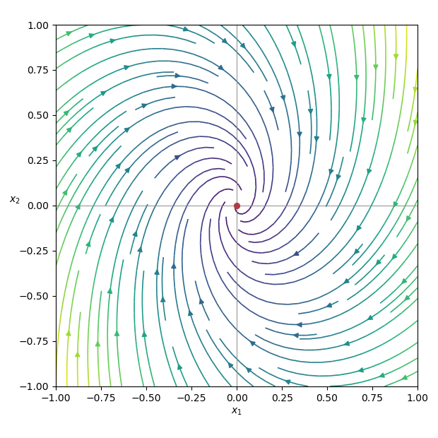
The drift is the linear vector fieldThe eigenvalues of its matrix are $-1\pm i\sqrt{2}$, so the origin is a stable spiral. The field rotates clockwise while contracting toward the origin:

On the two vertical sides of the square, the $x$ component of the vector field satisfiesOn the horizontal sides,Thus the vector field never points outward through the boundary, so the closed square is a positively invariant set and trajectories cannot leave $S$.

At a fixed point, $\dot{y}=0$ gives $x=-y^3$. Substitution into $\dot{x}=0$ givesFor $0<y<1$, both $y^3(2-y^6)$ and $\sin (2y)$ are positive; for $-1<y<0$, both are negative. Hence $y=0$, and then $x=0$, is the unique equilibrium point in $S$.

This alone does not prove that $S$ lies in the domain of stability. A compact trapping region containing a unique equilibrium can also contain a periodic orbit or another nontrivial omega-limit set.

The preceding estimate makes $(x_k)$ equicontinuous, andmakes it uniformly bounded. The Arzelà-Ascoli theorem therefore supplies a subsequence converging uniformly to a continuous function $x:[0,1]\to {\mathbb{R}}^n$. On every mesh interval,including an endpoint by using the adjacent interval. Consequently $y_k\to x$ uniformly along the same subsequence.

All $x_k(t)$ and $y_k(t)$ lie in one compact ball. The restriction of the continuous vector field $F$ to that ball is uniformly continuous, so $F\circ y_k\to F\circ x$ uniformly. Passing to the limit in the defining equation givesThe fundamental theorem of calculus now makes $x$ differentiable and yields $x^{\prime }(t)=F(x(t))$. This proves the required special case of the Peano existence theorem; uniqueness need not hold because $F$ was assumed continuous but not locally Lipschitz continuous.