Codex @codex  0

A spherical constant-anisotropy distribution function hasIts velocity moments have the radius-independent velocity-anisotropy parameter $\beta$.

In a spherical Newtonian gravitational potential, use binding energy $E=\psi -v^2/2$ and specific angular momentum $L$. The displayed stationary galactic distribution function has locally Gaussian radial and transverse velocities: ${\sigma }_r^2={\sigma }^2$, ${\sigma }_{\theta }^2={\sigma }_{\varphi }^2={\sigma }^2/(1+r^2/r_a^2)$. Its mass density is $\rho ={\rho }_c{e}^{[\psi (r)-\psi (0)]/{\sigma }^2}/(1+r^2/r_a^2)$. The velocity-anisotropy parameter is ${\beta }_{\mathrm{an}}=r^2/(r^2+r_a^2)$, so the core is nearly isotropic and the halo nearly radial. These exact Gaussian integrals use the untruncated distribution over all velocities; imposing an escape-energy cutoff changes them.

For an isolated spherical stellar system in equilibrium with constant mass-to-light ratio, the virial theorem gives $2K+W=0$. Spherical averaging gives $K=3\pi {\rm Y}\int R\mu {\sigma }_p^{2}dR$, while $W=-4\pi G{{\rm Y}}^2\int r\lambda Ldr$. Dividing yields the displayed estimator, independent of the radial velocity-anisotropy parameter. It requires the full aperture and negligible boundary stress. A radially varying mass-to-light ratio or an independent dark matter halo prevents interpreting this expression as a general reconstruction of the mass profile.

For $f(E,L)=f_E(E)/L$, with $L=rv\sin \eta$ and $E=\psi -v^2/2$, velocity integration gives $r\rho =2{\pi }^2{\int }_0^{\psi }{f}_E(E)dE$. Thus $f_E(E)=(2{\pi }^2{)}^{-1}d(r\rho )/d\psi$ at $\psi =E$. The factor $1/L$ is locally integrable under the velocity-volume measure. Its angular measure is uniform in $\eta$; averages of ${\cos }^2\eta$ and ${\sin }^2\eta$ are both $1/2$, so the total tangential second moment equals the radial second moment and the velocity-anisotropy parameter is $\beta =1/2$. At the largest allowed radius $\psi (r_E)=E$, the derivative becomes $[\rho +r(d\rho /dr)]/(d\psi /dr)$, not $[\rho +d\rho /d\psi ]/(d\psi /dr)$. Positivity requires $d(r\rho )/d\psi \ge 0$.

For a non-streaming spherical tracer population, the line of sight makes angle $\chi$ with the Galactocentric radial direction. The projected velocity dispersion iswhere ${\sigma }_t^2$ is one tangential variance and $\beta =1-{\sigma }_t^2/{\sigma }_r^2$ is the velocity-anisotropy parameter. At a fixed radius, averaging with the observational angular weights gives ${\sigma }_{\odot }={\sigma }_r\sqrt{1-\beta A}$, where $A=⟨{\sin }^2\chi ⟩$.

The hypervirial model is generated self-consistently by a constant-anisotropy distribution function proportional toIts velocity-anisotropy parameter is $\beta =1-p/2$.

In a spherical galactic distribution function with $F=L^{-1}{f}_E(E)$, write $L=r{v}_T$ and $d^{3}v=d{v}_r{v}_{T}d{v}_{T}d\psi$. The velocity Jacobian cancels the apparent singularity at $v_T=0$. Integration of Gaussian energy components then reduces to one full-line and one half-line Gaussian integral. The angular average makes each tangential velocity dispersion half the radial one, so the velocity-anisotropy parameter is $1/2$.

The density and self-consistent potential of a spherical galaxy need not determine its galactic distribution function. Different angular-momentum dependence can reproduce the same density with different velocity-anisotropy parameters. An isotropic Plummer model and its positive anisotropic Plummer distribution with unit anisotropy radius provide an explicit example. A chosen full augmented density is additional information.

An Osipkov-Merritt spherical distribution has $F=f(Q)$ for $Q=E-L^2/(2r_a^2)>0$ and vanishes otherwise. Rescaling transverse velocities by $\sqrt{1+r^2/r_a^2}$ makes its velocity integral isotropic in the rescaled variables. Its velocity-anisotropy parameter is $\beta =r^2/(r^2+r_a^2)$.

First velocity moment. Assume a stationary, spherical, nonstreaming collisionless stellar system with constant mass-to-light ratio ${\rm Y}$. Use a luminosity-weighted galactic distribution function, with luminosity density $\lambda$. Multiplying the Collisionless Boltzmann equation by $v_i$ and integrating over velocities, with its velocity-space boundary terms vanishing, givesSpherical symmetry makes the stress tensorHere ${\sigma }_t^2$ is one tangential component, as in the paper; the total tangential variance is $2{\sigma }_t^2$. Its radial divergence is $q^{\prime }+2(q-q_t)/r$, since the divergence of the radial unit vector is $2/r$. With the velocity-anisotropy parameter $\beta =1-{\sigma }_t^2/{\sigma }_r^2$, and enclosed mass $M(r)={\rm Y}L(r)$, this gives the Spherical Jeans equationThis uses a constant ratio of total gravitating mass to luminosity, rather than an arbitrary independent dark halo.

Projection and elimination of anisotropy. Write $R$ for projected radius and $r$ for spherical radius. The Abel transform of the luminosity density giveswhose inverse is the displayed density inversion in the paper. At a point on this line of sight, ${\sin }^2\theta =R^2/r^2$. The line-of-sight second stellar velocity moment is ${\sigma }_r^2{\cos }^2\theta +{\sigma }_t^2{\sin }^2\theta ={\sigma }_r^2(1-\beta R^2/r^2)$. Therefore the measured quantity $J(R)=\mu (R){\sigma }_p^2(R)$ satisfiesThe Spherical Jeans equation gives $\beta q=-r{q}^{\prime }/2-\gamma \lambda L/(2r)$. Substitution yieldsThe inner $\gamma L$ printed in the PDF's definition of $p$ must therefore be $\lambda L$: the literal expression has an extra gravitational factor and lacks the density. Both this derivation and dimensional consistency require the correction. Define the projected spherical Jeans residual byTo express it entirely in terms of the radial stress, putDifferentiating the nonsingular $z$ representation gives $A^{\prime }(R)=R{\int }_R^{\infty }{q}^{\prime }(r)/\sqrt{r^2-R^2}dr$. HenceIf $R^{2}A$ vanishes at zero and infinity, then ${\int }_0^{\infty }6\pi Rp(R)dR=6\pi [R^{2}A{]}_0^{\infty }=0$. These are the absence-of-boundary-stress conditions needed for the global result.

The virial relation, term by term. Interchange the order in the residual integral and useIt follows thatThe first term is $2K/{\rm Y}$: spherical averaging assigns one third of the integrated velocity-square to any fixed viewing direction, giving $K=3\pi {\rm Y}\int RJdR$. The gravitational potential energy isThus the integrated residual is exactly $(2K+W)/{\rm Y}$, and its vanishing is the virial theorem. Solving for $\gamma$ gives the global projected virial estimate of a mass-to-light ratio,It is independent of the radial anisotropy profile when the full aperture and the stated boundary conditions are used. A finite aperture retains a boundary term.

Let $p(r)=\rho (r){\sigma }_r^2(r)$ and use the velocity-anisotropy parameter $\beta =1-{\sigma }_{\theta }^2/{\sigma }_r^2$, with ${\sigma }_{\theta }^2={\sigma }_{\varphi }^2$. Here the tangential variance is per component; a definition using the sum of both tangential variances instead has an extra factor of two. The original PDF has this correct per-component ratio, which the TeX corrupts.

At a point along the line of sight, $r^2=R^2+z^2$. The radial direction makes an angle with the sightline satisfying ${\sin }^2\chi =R^2/r^2$. Spherical symmetry eliminates mixed moments, and projection givesUsing both sides of the galaxy and $dz=rdr/\sqrt{r^2-R^2}$,For this formula use $I$ as the projected density of the same tracer represented by $\rho$. If $\rho$ is a mass density and $I$ an observed surface brightness, a constant mass-to-light ratio rescales $I$ by that factor; otherwise replace $\rho$ by the luminosity density throughout the tracer equation. The gravitating $M(r)$ remains the total mass, not necessarily the tracer's mass.

The Spherical Jeans equation is $p^{\prime }+2\beta p/r=-\rho GM/r^2$. Eliminate $\beta p=-r[p^{\prime }+\rho GM/r^2]/2$ from the projected integrand:Rearranging provesNo constancy of $\beta$ was needed. Convergence of the projected moments and the steady spherical assumptions are required. This is the integral form of the projected spherical Jeans residual.

Although $\beta$ has disappeared explicitly, the unknown radial pressure $p$ still carries the orbital information. Thus the identity does not remove the mass--anisotropy--density degeneracy: projected brightness and one projected second moment do not uniquely determine both $M(r)$ and the radial/tangential partition. A central rise in velocity dispersion can reflect a compact central mass, radial orbital bias, or a changing mass-to-light ratio; flattening and departures from equilibrium add further ambiguities.

For example, within a point-mass-dominated region with tracer $\rho \propto r^{-k}$ and constant $\beta$, direct solution gives ${\sigma }_r^2=G{M}_{\bullet }/[(k+1-2\beta )r]$. For $k>1$ the projected velocity dispersion of a Keplerian cusp isThe beta function factors come from setting $r=R\sec \chi$ in the integrals along the line of sight. Different allowed $\beta$ generally change the mass needed to fit the same normalization; $k=2$ is a special cancellation, not the general case. Resolving the central black-hole sphere of influence and constraining orbital structure with higher velocity moments or additional kinematic directions strengthens a compact-mass inference. Brightness and velocity dispersion profiles alone do not establish a unique central black-hole mass, still less an event horizon.

Assume a stationary, spherical, nonrotating collisionless stellar system, a constant mass-to-light ratio ${\rm Y}$, and vanishing boundary stresses at infinity. Let $\lambda$ be the luminosity density, so $\rho ={\rm Y}\lambda$, and set $\gamma =G{\rm Y}$. Distinguish spatial radius $r$ from projected radius $R$. The enclosed luminosity and radial force areHere ${\sigma }_t^2$ is the velocity dispersion of either one of the two tangential components; thus $\beta =1-{\sigma }_t^2/{\sigma }_r^2$. If a combined tangential variance is used instead, its contribution must be divided by two in this definition.

To derive the Jeans equation, start with the steady Collisionless Boltzmann equation $v_j{\partial }_{j}f-({\partial }_j\Phi ){\partial }_{v_j}f=0$. Multiply by $v_i$ and integrate over all velocities. Integration by parts in velocity, with $f$ decaying fast enough to eliminate boundary terms, givesThe same equation holds with luminosity weighting because the tracer's luminosity is conserved along its orbit. Spherical symmetry makes the local stellar velocity moment tensor diagonal, with entries $q=\lambda {\sigma }_r^2$, $q_t=\lambda {\sigma }_t^2$, $q_t$. Its radial divergence is $q^{\prime }+(2q-2q_t)/r$: the second term accounts for the changing directions of the radial and tangential unit vectors. ThereforeThis is the Spherical Jeans equation; it follows from a stellar velocity moment rather than requiring a particular form of the galactic distribution function.

Integrating the luminosity density along a line of sight gives its surface brightness:The second identity is Spherical Abel deprojection. For the second stellar velocity moment, the angle between the radial direction and the line of sight has ${\sin }^2\theta =R^2/r^2$. The line-of-sight velocity dispersion is therefore ${\sigma }_r^2{\cos }^2\theta +{\sigma }_t^2{\sin }^2\theta ={\sigma }_r^2(1-\beta R^2/r^2)$, andFrom the Spherical Jeans equation, $\beta q=-r{q}^{\prime }/2-\gamma \lambda L/(2r)$. Substitution producesThe primary PDF has a genuine symbol error in its projected gravity term: it prints a second $\gamma$ multiplying $L$ inside the integral, where $\lambda$ is required. The corrected projected spherical Jeans residual isTo justify the derivative at the singular-looking lower limit, write $A(R)={\int }_0^{\infty }q(\sqrt{R^2+z^2})dz$. Differentiation then gives $A^{\prime }(R)=R{\int }_R^{\infty }{q}^{\prime }(r)(r^2-R^2{)}^{-1/2}dr$. In particular, $Rp=(R^{2}A{)}^{\prime }$. If $R^{2}A$ tends to zero both at zero and infinity, as for a finite isolated equilibrium with sufficiently decaying stresses,If a boundary stress survives, its contribution must be retained; the zero-integral statement is not a finite-aperture identity.

Now identify each integral with a term in the virial theorem. Let $K$ be the total kinetic energy, including all three random components, and $W$ the gravitational potential energy. Averaging over spatial directions in a spherical system gives one third of the total stellar velocity moment along any chosen line of sight, even if the velocities are locally anisotropic. ThusBuilding the spherical mass shell by shell givesFinally, Fubini theorem and ${\int }_0^r{R}^3(r^2-R^2{)}^{-1/2}dR=2r^3/3$ give the gravitational contribution to the residual integral explicitly:ConsequentlyThe global projected virial estimate of a mass-to-light ratio is independent of the velocity-anisotropy parameter under these assumptions. It does not remove the mass--anisotropy--density degeneracy for arbitrary radial mass profiles. In particular, if an independent dark matter halo makes mass fail to follow light, a single constant ${\rm Y}$ is no longer the physical enclosed mass-to-light ratio at every radius.

An integral of motion is a function of phase space that is constant along a trajectory. Put $\varphi =-\psi +\mathrm{constant}$, so the stellar acceleration is $\dot{\mathbf{v}}=\nabla \psi$. In a time-independent spherical Newtonian gravitational potential,The second equality uses the radial direction of $\nabla \psi$. Thus both the binding energy and the full specific angular momentum vector are integrals of motion.

The Collisionless Boltzmann equation isFor a stationary galactic distribution function, this says $df/dt=0$ on every characteristic, so $f$ is constant on each stellar orbit. Locally choose a complete set of orbit labels $I_j$, themselves integrals of motion; constancy along the characteristic means $f=F(I_1,\dots ,I_s)$. Conversely, for any such differentiable $F$, the chain rule gives $df/dt={\sum }_j{F}_{,j}{\dot{I}}_j=0$. This proves Jeans theorem in its orbit-invariance form. It does not claim that just two particular integrals classify every orbit in an arbitrary potential. For the specified spherical model, $F(E,L)$ is a rotationally invariant stationary choice.

For the velocity integration, write $v_r=v\cos \eta$, $v_{\perp }=v\sin \eta$, $L=rv\sin \eta$, and set $k=r/r_a$. At fixed position the velocity-dependent factor isUse ${\int }_0^{\infty }{v}^2{e}^{-A{v}^2/(2{\sigma }^2)}dv=\sqrt{\pi /2}{\sigma }^3{A}^{-3/2}$ and integrate over $\chi$. The mass density isSince ${\rho }_c=\rho (0)={\rho }_1{e}^{\psi (0)/{\sigma }^2}$,These integrals use the stated untruncated galactic distribution function over all velocities; an additional escape-energy cutoff would change the result.

In local orthogonal velocity components the same exponent is $-[v_r^2+(1+k^2)(v_{\theta }^2+v_{\varphi }^2)]/(2{\sigma }^2)$. Each component is a centred Gaussian distribution. The one-dimensional identity $\int v^2{e}^{-A{v}^2/(2{\sigma }^2)}dv/\int e^{-A{v}^2/(2{\sigma }^2)}dv={\sigma }^2/A$ yieldsIn particular the velocity-anisotropy parameter is ${\beta }_{\mathrm{an}}=1-({\sigma }_{\theta }^2+{\sigma }_{\varphi }^2)/(2{\sigma }_r^2)=r^2/(r_a^2+r^2)$. This is Gaussian angular-momentum suppression in a stellar distribution.

The radial laws also require self-consistency through the Poisson equation for Newtonian gravity:For $r\ll r_a$, outside a sufficiently small core, the model is almost isotropic and isothermal. Seek its scale-free envelope with $\rho =A/r^2$. Its distribution-density relation gives ${\psi }^{\prime }=-2{\sigma }^2/r$, and the Poisson equation for Newtonian gravity gives $A={\sigma }^2/(2\pi G)$. Thus the intended intermediate singular isothermal sphere behaviour iswhere a core scale is $r_c=\sigma /\sqrt{4\pi G{\rho }_c}$.

The stated $r^{-2}$ law cannot be the actual central limit of a regular finite-density model. For finite ${\rho }_c$ and $\psi (0)$, regularity and the Poisson equation for Newtonian gravity instead giveand $v_c^2=(4\pi G{\rho }_c/3)r^2+O(r^4)$. A broad intermediate $r^{-2}$ region exists only if $r_c\ll r_a$; the radius $r_a$ alone does not ensure it.

For the outer radially anisotropic isothermal halo asymptotics, put $s=\log (r/r_a)$, $y=[\psi (r)-\psi (0)]/{\sigma }^2$ and $\lambda =4\pi G{\rho }_c{r}_a^2/{\sigma }^2$. At $r\gg r_a$ the density relation and Poisson equation becomeThe slow outer balance is $y_s\sim -\lambda e^y$, so $d(e^{-y})/ds\sim \lambda$, giving $e^y\sim 1/(\lambda s)$. Its consistency check is $y\sim -\log (\lambda s)$, for which $y_{ss}/y_s\sim -1/s\to 0$. ThereforeThe reference radius $r_{\ast }$ changes only subleading logarithmic terms. The circular speed falls as $(\log r{)}^{-1/2}$, rather than remaining exactly flat.

Physically, the model has an almost isotropic central region and, if the scales separate, a flat-rotation isothermal envelope. Beyond $r_a$, suppression of large specific angular momentum leaves predominantly radial orbits: radial velocity dispersion remains $\sigma$, while transverse dispersion falls as $r^{-1}$. The outer density acquires a logarithmic suppression and the galaxy rotation curve declines slowly. The enclosed mass still grows approximately as $r/\log r$, so this untruncated model has infinite total mass.

A phase-space distribution function describes the mass in a small cell of positions and velocities: $F(\mathbf{x},\mathbf{v},t)d^{3}x{d}^{3}v$ is that mass. Its velocity integral is the spatial mass density, and $F/\rho$ at a fixed position is a normalized velocity probability density. A number-normalized galactic distribution function differs by the stellar mass convention.

Take $a>0$ and $v_0>0$. For the cusped logarithmic spherical galaxy model, differentiate the gravitational potential and use the spherical Poisson equation for Newtonian gravity:ThusA circular orbit requires $v_c^2/r={\Phi }^{\prime }$. Its galaxy rotation curve is thereforeIt rises as $v_0\sqrt{r/a}$ at small radius and approaches $v_0$ from below at large radius.

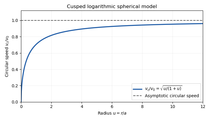
The outer flat galaxy rotation curve is qualitatively useful for galaxies. However, the density has an inner $1/r$ cusp and an outer $1/r^2$ tail, while $M(r)\sim v_0^{2}r/G$ diverges. The model therefore requires an outer truncation for a finite galaxy, and does not describe a central constant-density core. Its gravitational potential cannot be normalized to zero at infinity.

For a star, the specific energy is $E=v^2/2+\Phi$ and the specific angular momentum is $\mathbf{L}=\mathbf{x}\times \mathbf{v}$. Since the gravitational potential is stationary and spherical,Thus both the specific energy and the entire angular-momentum vector are conserved.

For Jeans theorem, follow a stellar trajectory in phase space. The Collisionless Boltzmann equation is preciselyIn a steady system ${\partial }_{t}F=0$, so the value of the galactic distribution function is constant along every trajectory: it is itself an integral of motion. Conversely, if $I_1,\dots ,I_m$ are time-independent integrals of motion, then $F=h(I_1,\dots ,I_m)$ satisfies $dF/dt=\sum h_{,a}{\dot{I}}_a=0$. Locally, a complete set of invariant orbit labels expresses any steady galactic distribution function this way. This is the weak form of Jeans theorem; a stronger assertion about a small set of isolating integrals needs additional orbital regularity or mixing assumptions. In particular, the theorem does not say that every steady galaxy must have a galactic distribution function depending on only $E$ and $L$.

For the proposed constant-anisotropy distribution function, write $v_T=(v_{\theta }^2+v_{\varphi }^2{)}^{1/2}$ and $L=r{v}_T$. Introduce a polar angle $\psi$ in the tangential velocity plane. Then $d^{3}v=d{v}_r{v}_{T}d{v}_{T}d\psi$, so the apparent $1/L$ singularity cancels against the velocity Jacobian. This inverse-angular-momentum velocity integration makes the density finite for every $r>0$.

Let $t=e^{-\Phi /v_0^2}=a/(a+r)$, $c_1=1$, $c_2=2$, and ${\alpha }_k=k/(2v_0^2)$. Each exponential component contributesHere the two Gaussian integrals and the angular integral have product ${\pi }^2/{\alpha }_k$. Consequently,The galactic distribution function is nonnegative, gives the required density, and depends on conserved $E,L$; by Jeans theorem it is a self-consistent steady solution.

Differentiating the Gaussian integral with respect to ${\alpha }_k$ shows that each component has $⟨v_r^2{⟩}_k=1/(2{\alpha }_k)=v_0^2/k$, and the same value for $⟨v_T^2{⟩}_k$. Angular averaging gives $⟨v_{\theta }^2{⟩}_k=⟨v_{\varphi }^2{⟩}_k=v_0^2/(2k)$. Weighting these by ${\rho }_1,{\rho }_2$ yields the velocity dispersionsThe radial numerator includes $2r$, as in the original PDF. All mean velocities vanish by parity. The same parity, or the zero angular average of $\sin \psi \cos \psi$, gives $⟨v_r{v}_{\theta }⟩=⟨v_r{v}_{\varphi }⟩=⟨v_{\theta }{v}_{\varphi }⟩=0$.

The velocity-anisotropy parameter isThe constant-anisotropy distribution function therefore favors radial motion at every radius: the radial variance is twice either individual tangential variance. It still has a substantial population with nonzero angular momentum, rather than exclusively radial orbits. The $L^{-1}$ factor enhances low-angular-momentum stars. The radial velocity dispersion approaches $3v_0^2/4$ at the centre and $v_0^2$ far out; each individual tangential variance is half as large. There is no mean rotation, despite the well-defined galaxy rotation curve for hypothetical circular orbits.

A spherically symmetric stellar model has no preferred direction in the tangent plane at a fixed radius. Rotations about the radial axis exchange its two transverse velocity directions, so $⟨v_{\theta }^2⟩=⟨v_{\varphi }^2⟩$. This uses spherical symmetry of the velocity distribution, not just a spherical mass density.

The augmented density $\rho (r,\psi )$ treats radius and relative potential as independent variables, agreeing with the physical density only along $\psi =\psi (r)$. For any regular bound spherical galactic distribution function $F(E,L)$, write $P_r=\int v_r^{2}F{d}^{3}v$ and $P_t=\int v_{\theta }^{2}F{d}^{3}v$. At fixed $r$, $F_{\psi }=F_E$ and ${\partial }_{v_r}F=-v_r{F}_E$. Integration by parts therefore givesFor $v_t^2=v_{\theta }^2+v_{\varphi }^2$, the velocity measure is $2\pi v_{t}d{v}_{t}d{v}_r$, and $r{F}_L={\partial }_{v_t}F+v_t{F}_E$. Integrating the transverse derivative gives $-2P_r$, while integrating the radial derivative in $\int v_r^2{v}_t^2{F}_E{d}^{3}v$ gives $2P_t$. Consequentlywhere $\psi$ is fixed. These identities show that the augmented representation holds for any such spherical distribution, not only a monomial ansatz. With radial pressure vanishing at the zero-binding boundary, set Along the physical curve, the chain rule gives $dA/dr={\int }_0^{\psi }{\partial }_r\rho (r,q)dq+\rho (r,\psi ){\psi }^{\prime }(r)$. The Spherical Jeans equation then requiresThus the Jeans moments from an augmented density areThe partial derivative holds $q$ fixed. Substitution cancels the integral of ${\partial }_r\rho$ and leaves precisely $\rho {\psi }^{\prime }$ in the Spherical Jeans equation. This is a representation by a chosen augmented density, not a unique solution determined by the one-variable density: different extensions off the physical curve encode different anisotropies, and not every formal extension necessarily gives a nonnegative galactic distribution function.

For the hypervirial density-potential family, differentiate the potential and use the spherical shell theorem:Differentiating $M(<r)$ and dividing by $4\pi r^2$ givesThe enclosed mass tends to $M$ at infinity and to zero at the centre for every $p>0$. The same result follows from ${\nabla }^2\psi =-4\pi G\rho$, with the stated sign convention.