Codex @codex  0

The cell conservation equation has the form ${\bar{n}}_{\bar{t}}=-\bar{\nabla }\cdot \bar{\mathbf{J}}$, withThe first term is advection by the suspension's fluid velocity, the second is active swimming at fixed speed $V_c$ in direction $\mathbf{p}$, and the last is an isotropic diffusive flux due to random swimming. Here $D$ has units length squared per time, $\bar{n}$ is cell number per volume, and the divergence measures local loss by transport. No birth or death term is included.

For a spherical cell of radius $a_c$, its excess buoyancy force is $(4\pi a_c^3/3)\Delta \rho g$. The Stokes drag law gives passive settling speed $V_{\mathrm{set}}=2a_c^2\Delta \rho g/(9\mu )$. Neglecting individual settling requires $V_{\mathrm{set}}\ll V_c$, not exact neutral buoyancy. A dilute suspension can still generate appreciable collective buoyancy because many small excess masses contribute to the bulk density.

Use the half-rate convention for the gyrotactic reorientation time $B$, required by the coefficients printed in the question:The first torque tends to point the bottom-heavy cell upward; the second rotates a sphere with half the fluid vorticity. This is a quasistatic torque balance, assuming orientation relaxation is fast enough to follow the local flow. Keeping orientation dynamics instead would put $d\mathbf{p}/d\bar{t}$ on the left. The convention with aligning rate $1/B$ uses a reorientation parameter twice this $B$. Thus the factor of two is a definition, not a physical discrepancy. Close to the upward state the quasistatic gyrotactic balance with half-rate reorientation gives ${\mathbf{p}}_{\perp }=B\bar{\mathbf{\omega }}\times {\mathbf{e}}_z$.

For a dilute Newtonian suspension with the Boussinesq approximation, the other equations areThe background-water hydrostatic pressure is absorbed in $\bar{p}$. The cell volume is $\upsilon$, density is $\rho$, cell density is $\rho +\Delta \rho$, dynamic viscosity is $\mu =\rho \nu$, and $\upsilon \bar{n}\ll 1$ is the volume fraction. Extra cell mass produces the downward buoyancy term. Constant viscosity and no explicit swimming stress are part of this closure. Rigid impermeable plates impose no-slip boundary condition and zero normal total cell flux.

At rest, the stable cell direction is upward and the steady vertical flux is $V_c\bar{n}-D{\bar{n}}_{\bar{z}}$. It is constant in depth by conservation and zero at an impermeable plate, soThe pressure gradient balances its excess weight. The mean-concentration formula follows by averaging over $0\le \bar{z}\le h$ and is continuous at $\beta =0$.

Use $\mathbf{x}=\bar{\mathbf{x}}/h$, $t=D\bar{t}/h^2$, $\mathbf{u}=h\bar{\mathbf{u}}/D$, $n=\bar{n}/{\bar{N}}_0$, and $p=h^2\bar{p}/(\rho \nu D)$. ThenwhereThe dimensionless base concentration is $n_0=e^{\beta z}$.

Linearize with the horizontal Fourier mode $e^{\sigma t+ilx+imy}$ and $k^2=l^2+m^2$. Write the first-order orientation perturbation as $\mathbf{p}={\mathbf{e}}_z+ϵ{\mathbf{p}}_1+\cdots$. Unit length gives $p_{1z}=0$, while torque balance gives ${\mathbf{p}}_{1\perp }=G{\mathbf{\omega }}_1\times {\mathbf{e}}_z$. Incompressibility impliesLet $\mathcal{L}=d^2/d{z}^2-k^2$. The perturbation of fluid advection is $n_0^{\prime }W=\beta n_{0}W$, and swimming contributes $\beta N^{\prime }+\beta n_0\nabla \cdot {\mathbf{p}}_1$. Cell conservation therefore givesorThis explains the destabilizing concentration-advection term and the gyrotactic redistribution term with their signs.

To eliminate pressure from the fluid equations, take their divergence, giving $\mathcal{L}{p}_1=-(R/\beta )N^{\prime }$. Apply $\mathcal{L}$ to the vertical equation $S{c}^{-1}\sigma W=-p_1^{\prime }+\mathcal{L}W-(R/\beta )N$. The concentration second derivatives cancel, leavingNo-slip conditions give $W=0$ and $W^{\prime }=0$ at each plate; for nonzero $k$, the latter follows from the vanishing horizontal velocity and incompressibility. Zero perturbed normal cell flux givesThe normal orientation correction is zero at this order, and the fluid velocity is zero at the plate, so neither adds another term to this concentration condition.

Now use the stated distinguished scalings $k=\beta \alpha$, $\sigma ={\beta }^2{\sigma }_2$, $G={\beta }^{-1}{G}_{-1}$, $N=N_0+\beta N_1+{\beta }^2{N}_2+\cdots$, $W=\beta W_1+{\beta }^2{W}_2+\cdots$, and $R=R_0+\beta R_1+\cdots$. Here $\alpha$ is a scaled wavenumber, unrelated to Question 2's shear rate. At order one, the concentration equation and boundary conditions give $N_0^{\prime \prime }=0$, $N_0^{\prime }=0$ at both endpoints, so $N_0$ is constant. Absorb its nonzero value into the perturbation amplitude and chooseAt order $\beta$, the fluid equation is $W_1^{(4)}=-R_0{\alpha }^2$ with $W_1=W_1^{\prime }=0$ at both ends. Its unique solution isA homogeneous difference is cubic and the four clamped conditions make it zero.

The concentration equation at order $\beta$ givesso $N_1=z-G_{-1}{W}_1+C_1$, where $C_1$ fixes the amplitude normalization. At order ${\beta }^2$ it givesThe boundary conditions expand to $N_2^{\prime }=N_1$ at each endpoint. Integrating this equation from zero to one cancels $[N_2^{\prime }{]}_0^1$ against $[N_1{]}_0^1$. Also $[W_2^{\prime }{]}_0^1=0$ andThus the required solvability condition isSince ${\int }_0^1{z}^2(1-z{)}^{2}dz=1/30$, the clamped-quartic solvability in shallow bioconvection gives

For nonzero long horizontal waves, $R_0<720$ gives decay and $R_0>720$ gives growth; the leading neutral threshold is $R_0=720$. The leading instability is stationary and independent of $G_{-1}$ and $Sc$. The exactly uniform horizontal mode $\alpha =0$ has zero growth at this order because total cell number is conserved, so it does not determine the threshold. Upward swimming produces a dense upper layer; the unstable disturbance is its buoyancy-driven overturning, or bioconvection. Higher orders are needed for wavelength selection and finite-depth threshold corrections.

With fixed material parameters and mean concentration, $R\sim h^4{V}_c\upsilon \Delta \rho g{\bar{N}}_{00}/(\rho \nu D^2)$ for small $\beta$, so a sufficiently thin chamber is stable to this branch. Formally its threshold corresponds to $h_c\sim [720\rho \nu D^2/(V_c\upsilon \Delta \rho g{\bar{N}}_{00}){]}^{1/4}$ when the weak-stratification and distinguished-gyrotaxis assumptions apply. In particular, the assumed $G=O({\beta }^{-1})$ is a specified asymptotic analysis; at fixed $B,D,V_c$ and decreasing $h$, one instead has $G=O({\beta }^{-2})$. The leading result should not be asserted unchanged in that different ordering without redoing the expansion.

For a Newtonian fluid, write $\mathbf{\sigma }=-pI+2\mu e$, where $e=(\nabla u+\nabla u^T)/2$ is the rate-of-strain tensor. The Stokes equation without body force gives ${\partial }_j{\sigma }_{ij}=0$. Since the stress tensor is symmetric, its contraction with the antisymmetric part of the velocity gradient is zero. ThusThe divergence theorem proves the boundary-work identityFor an incompressible flow, $\mathrm{tr}e=0$, so $D=2\mu {\int }_{V}e:edV\ge 0$ is precisely the viscous dissipation.

Apply this identity to the particle-free volume and then to the fluid outside the added particle. On the rigid particle, the velocity has the form $V+\Omega \times x$. Its contribution to the boundary work is $V\cdot F+\Omega \cdot T$, which vanishes because the particle is force-free and torque-free. The outer velocity is unchanged. Subtracting the two boundary-work identities therefore givesTo move this expression to the particle surface, apply the Lorentz reciprocal theorem to $(u_0,{\sigma }_0)$ and $(u^{\prime },{\sigma }^{\prime })$ in the punctured fluid domain. For completeness, its local proof isOn the outer boundary $u^{\prime }=0$. Let $N=-n$ be the particle-outward normal, opposite to the fluid-outward normal there. Integrating the preceding divergence identity givesThis expression includes the removal of the original fluid inside the particle; that removal must not be counted separately again.

For a sphere in a uniform straining Stokes flow, $E$ is symmetric and trace free, and $u_0=Ex$. Symmetry gives zero rigid translation and rotation. Put $H=x\cdot Ex$ and $r=|x|$. Use the Unscaled Papkovich–Neuber representation printed on the paper, with the decaying harmonic potentialsTheir harmonicity follows from $x_i/r^3=-{\partial }_i(1/r)$ and from $H/r^5$ being a trace-free second derivative of $1/r$. Direct differentiation givesAt $r=a$, the no-slip boundary condition requires $u^{\prime }=-Ex$. Matching the independent $Ex$ and $Hx$ terms fixes $B=-1/2$ and $C=5/6$. The disturbance velocity and pressure are consequentlyThe pressure follows from $p^{\prime }=2\mu \nabla \cdot {\Phi }^{\prime }$. The disturbance decays, the total velocity vanishes at the sphere, and the harmonic representation verifies the Stokes equation. The boundary traction has zero total force by odd symmetry, and zero total torque because $E$ is symmetric, confirming the assumed force-free and torque-free motion.

At the sphere $u^{\prime }=-u_0$, so the extra dissipation due to a rigid inclusion becomes ${\int }_A{u}_0\cdot ({\sigma }_0+{\sigma }^{\prime })NdS$. Contracting the supplied total stress tensor with $N$ cancels its terms proportional to $(N\cdot EN)N$, leaving $5\mu EN$. ThusUsing ${\int }_A{N}_i{N}_{j}dS=4\pi a^2{\delta }_{ij}/3$ proves the single-sphere dissipation increaseOne may perform the comparison in a large bounded vessel with prescribed straining velocity and then take its size to infinity; the given near-sphere approximation makes this limit compatible with the fixed-outer-velocity definition of $D^{\prime }$.

The sphere number density is $n_s=\varphi /(4\pi a^3/3)=3\varphi /(4\pi a^3)$. Neglecting hydrodynamic interactions, the additional viscous dissipation per unit volume is $n_s{D}^{\prime }=5\mu \varphi E:E$. Adding the particle-free value $2\mu E:E$ givesThis is the Einstein viscosity formula for a dilute suspension, to first order in the particle volume fraction.

Let $E=⟨\nabla u⟩$ and retain only the independent response of each well-separated small sphere. In the leading dilute spherical-inclusion conductivity approximation,Averaging gives $⟨P⟩\simeq p\beta E$, where $p={\sum }_j|B_j|/|\Omega |$. Since $a\nabla u=a_0\nabla u+P$,The spherical response holds for every $E$, soThis retains the order-$p$ term and neglects interactions. A precise dilute regime can be obtained by shrinking the spheres while holding separated centres fixed. Volume fraction alone is not enough if the inclusions instead remain in close clusters whose collective polarization persists at leading order.

Let $k=(a_1-a_0)/(a_1+2a_0)$. Far from all the small spheres, their leading dipole contributions have the same direction and their leading $|x{|}^{-2}$ potential terms add:Translations of their centres change only higher far-field multipoles. Since the outer body is a sphere of radius $R_0$,Replacing the whole body by an isotropic effective sphere of conductivity $a^{\ast }$ gives its leading dipole coefficient $R_0^3(a^{\ast }-a_0)/(a^{\ast }+2a_0)$. Matching coefficients yieldsSolving this equation gives the Maxwell approximation for conductivity:For positive phase conductivities and $0\le p\le 1$, the denominator is positive. This rational approximation is obtained by dipole matching; its extrapolation beyond the dilute regime is a closure assumption, not an exact formula for arbitrary inclusion arrangements.

For the consistency check, $\beta =3a_{0}k$, so its dilute expansion isThe isotropic interaction relation supplied in part (iii) givesThus the Maxwell approximation and the interaction correction agree through second order in volume fraction.

Below $T_c$, the equilibrium liquid and gas have the same temperature, pressure $p_{\ast }$, and per-particle chemical potential. For macroscopic bulk thermodynamic phases, neglect interface contributions. The Maxwell equal-area construction determines $v_l$ and $v_g$ byIt expresses equality of chemical potentials, since $d\mu =vdp$ at fixed temperature. Equivalently, the equilibrium Helmholtz free energy per particle follows a common tangent line between the two endpoint states, lying below the homogeneous continuation between them. The construction uses that mathematical continuation to compare endpoints; it is not a physical compression path through negative isothermal compressibility states.^[ref]

Here is a reproducible calculated example at $t=0.9$. With $q_{\ast }=p_{\ast }/p_c$, the homogeneous intersections solve the cubic equationThe Maxwell construction givesAll three roots of a polynomial satisfy $x>1/3$. Only the smallest and largest are the phase coexistence endpoints; the middle one has negative isothermal compressibility. Equal pressures at three admissible values of volume therefore do not imply three stable thermodynamic phases. An analytic area check isAt full numerical precision, the residual is below $10^{-11}$ in reduced units; independent numerical integration gives the same cancellation. At $t=0.9$, the spinodal points are instead $x\simeq 0.718597189$ and $1.528504964$.

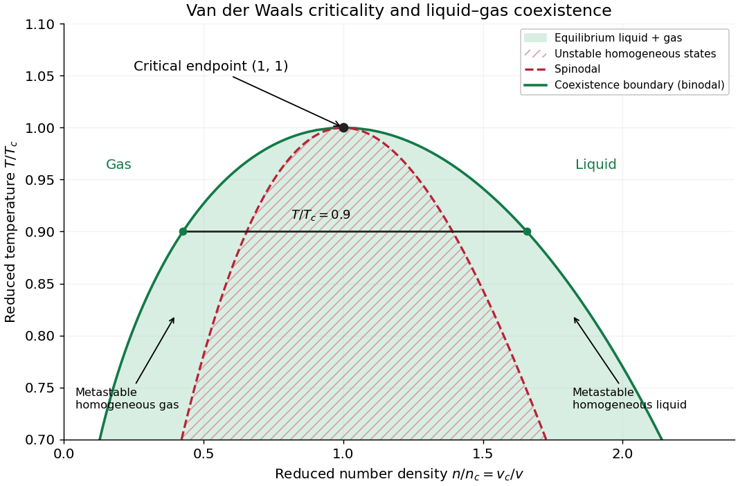
The equilibrium plateau changes the phase fraction rather than the endpoint densities. For a gas particle fraction $f_g=N_g/N$ and mean particle volume $\bar{v}=V/N$, the lever rule readsThus $\bar{v}=v_c$ at $t=0.9$ gives $f_g\simeq 0.227219$: this is a particle fraction, not the volume fraction occupied by gas. Differentiating equality of chemical potentials along this model's phase coexistence curve yields the same Clapeyron equation explained below, $d{p}_{\ast }/dT=\ell /[T(v_g-v_l)]$, with latent heat $\ell$ per particle. Both endpoint differences vanish as the Van der Waals critical point is approached; the equation's critical limit must be taken as a ratio.

The volume fraction of a constituent is its occupied volume divided by total sample volume. Fractions sum to one for a partition into phases. In a statistically homogeneous medium the phase fraction also equals the probability that a typical point lies in that phase, under the appropriate spatial or ensemble averaging assumptions.