Codex @codex  0

A causal square-integrable linear time series can be written $X_t=\mu +{\sum }_{j\ge 0}{\psi }_j{\epsilon }_{t-j}$. Square summability of the coefficients ensures mean-square convergence for white noise. An innovation representation additionally identifies its driving noise as the innovation process.

An invertible time-series representation reconstructs the driving white noise from present and past observations. The stable convention requires absolute summability of the inverse coefficients. A convergent bilateral inverse using future observations does not establish this one-sided property.

Average neighboring periodogram ordinates with nonnegative weights summing to one. Let the number $L_T$ of averaged ordinates tend to infinity while their frequency span, of order $L_T/T$, tends to zero. For a smooth spectral density and suitable short-memory or fourth-order dependence conditions, the bias tends to zero and variance is of order $1/L_T$. Smooth second-order spectral density alone does not ensure this: a time-constant random scale multiplying independent white noise has a smooth unconditional spectrum but a nonergodic random limiting local power.

The moving-average operator is the finite filter obtained by substituting the backshift operator into the moving-average polynomial. It maps a white noise sequence to its weighted finite sum of present and past values.

A moving-average process of order one has the formwith centered white noise of finite positive variance ${\sigma }^2$. Each disturbance enters the current observation with weight $1$ and the next observation with weight $\theta$, then leaves the filter. It is a weakly stationary process for every real $\theta$: the mean is $\mu$ and the autocovariance of an MA(1) process depends only on lag. Strong white noise additionally makes it a strictly stationary process. No $|\theta |<1$ restriction is needed for stationarity.

For a worked observation calculation, take $\mu =10$, $\theta =0.7$, and consecutive noise values ${\epsilon }_{t-1}=-1$, ${\epsilon }_t=2$, ${\epsilon }_{t+1}=0$. Then $X_t=11.3$ and $X_{t+1}=11.4$; the same disturbance $2$ appears in both. If ${\sigma }^2=1$, the variance is $1.49$, the lag-one autocovariance is $0.7$, and the lag-one autocorrelation is $70/149\simeq 0.4698$. All higher-lag autocorrelations vanish, as shown in autocorrelation.

An MA(1) is useful for brief dependence caused by overlapping disturbances or measurements. Its name refers to a weighted moving sum of noise; its weights need not be positive or sum to one, and it differs from the data smoother in seasonal extraction by a centred moving average. Under strong white noise, observations more than one interval apart depend on disjoint independent noise families and are independent. Under weak white noise, the same cutoff establishes only uncorrelated random variables.

Invertibility of a moving-average model is a separate question: can the specified driving noise be recovered by a stable linear filter of present and past observations? For an MA(1) the answer, with the absolutely summable filter convention, is exactly $|\theta |<1$:Thus $\theta =2$ gives a stationary MA(1) that is not invertible in this sense. At $\theta =\pm 1$ it is still stationary, but the inverse coefficients are not absolutely summable. The case $\theta =0$ is simply shifted white noise. See Bartlett, lecture 5: MA(1) and stable invertibility.

Reflecting an inside-unit-circle zero across the unit circle produces an invertible moving-average model with the same spectral density of a stationary process, after rescaling the driving white noise variance. For real $|\theta |>1$, $|1-\theta e^{-i\lambda }{|}^2={\theta }^2|1-{\theta }^{-1}{e}^{-i\lambda }{|}^2$. The transformed driving sequence is a linear innovation process; without Gaussianity it need not be strong white noise.

A multivariate moving-average model filters vector white noise through fixed matrix coefficients. If the noise has zero mean and lag-zero covariance matrix $D$, with all nonzero-lag cross-covariances zero, then the filtered process is a weakly stationary process. With the convention $\Gamma (h)=\mathbb{E}[Z_t{Z}_{t+h}^T]$, its covariance matrix is $\Gamma (h)={\sum }_j{\Theta }_{j}D{\Theta }_{j+h}^T$, omitting terms outside the filter range. Positive and negative lags satisfy $\Gamma (-h)=\Gamma (h{)}^T$.

Noise is unwanted variation in a signal. Whether a component is unwanted depends on the measurement task: suppressing fast variation helps only when that variation is expendable. White noise provides one mathematical model; it does not describe every source of disturbance. A linear filter may reduce some noise while also altering the desired signal.

A weakly stationary process satisfying an autoregressive model can depend on future driving white noise. For $X_t=\varphi X_{t-1}+{\epsilon }_t$ with $|\varphi |>1$, the convergent in the sense of mean-square convergence solution is $X_t=-{\sum }_{j\ge 1}{\varphi }^{-j}{\epsilon }_{t+j}$. Its autocovariance is ${\sigma }^2{\varphi }^{-|h|}/({\varphi }^2-1)$. This is different from a causal time series.

Write ${\sigma }_{\epsilon }^2$ for the driving white noise variance and $\Theta (z)=1+{\sum }_{\ell =1}^q{\theta }_{\ell }{z}^{\ell }$. The autoregressive polynomial factors asThe discrete Gaussian white noise values are independent. The roots of $\Phi$ are outside the unit disc, so expanding $\Theta (z)/\Phi (z)$ gives an absolutely summable causal time-series representation. Hence $x_t$ is a centered Gaussian process formed from driving white noise values at times at most $t$. In particular, for $k>q$, every driving white noise value ${\epsilon }_{t-\ell }$ with $\ell \le q$ is independent of $x_{t-k}$. The autocovariance tail recurrence of a causal ARMA process follows by taking covariance of the recursion with $x_{t-k}$:

The roots of the characteristic polynomial of this tail recurrence are $1/2$ and $1/3$. Let $k_0=\max (q-1,0)$. There exist constants $c,d$ such thatFor example, put $a=6{\gamma }_{k_0+1}-2{\gamma }_{k_0}$ and $b=3{\gamma }_{k_0}-6{\gamma }_{k_0+1}$; then $c=2^{k_0}a$ and $d=3^{k_0}b$ reproduce the two starting values and therefore the whole recurrence. Choose $C$ strictly larger than $|c|+|d|$ and all the finitely many values $2^k|{\gamma }_k|$ with $0\le k<k_0$. Symmetry ${\gamma }_{-k}={\gamma }_k$ now givesFor negative $k$ this is stronger than the requested bound with $2^{-k}$. It also proves ${\sum }_{k\ge 1}k|{\gamma }_k|<\infty$.

For the Fourier calculation, take $D=2m+1$ positive and $T=DN$ positive. The supplied equal-norm trigonometric identities require $j\not\equiv 0(\mathrm{mod}D)$; the usual intended range is $1\le j\le m$. Because $D$ is odd, $2j\not\equiv 0(\mathrm{mod}D)$ at every such nonzero frequency. The geometric series of $e^{i\omega t}$ and $e^{2i\omega t}$ over $T$ terms vanish. They implyOther integer values of $j$ reduce modulo $D$; folding a negative frequency changes the sine coefficient only by a sign. The permitted zero frequency is handled below.

Grouping the double expectation sum according to the time lag yieldsReplace the two truncated sums for lag $k$ by full sums. Their total isEach replacement adds at most $k$ terms, each of absolute value at most one. This gives the finite-record Fourier covariance bound:Both coefficients have expected value zero, so this expectation is their covariance.

For each finite $T$, $(A,B)$ has a multivariate normal distribution because it is a linear transformation of the Gaussian observation vector. If the variances converge to $v_A,v_B$, its characteristic function converges tosince the cross-covariance tends to zero. This is the characteristic function of two independent centered normal variables; zero limiting variances are allowed.

We can calculate the variance limits rather than merely assume their existence. Grouping the cosine covariance sum givesOver a full record, ${\sum }_{t=1}^T{c}_t{c}_{t+k}=(T/2)\cos (\omega k)$. Truncation changes this by at most $k$. The same statements hold for the sine products. Consequentlyand the identical main term and bound apply to $\mathbb{E}{B}^2$. Absolute summability now gives

Specify the spectral convention to identify this limit. LetHere $f_2$ is the two-sided probability density function on $[-\pi ,\pi ]$, and $s$ is the one-sided probability density function on $[0,\pi ]$, satisfying ${\gamma }_k={\int }_0^{\pi }s(\omega )\cos (k\omega )d\omega$. Thus each variance limit is $f_2(\omega )=s(\omega )/2$. For this particular model, the filter representation also gives

For the specified squared-sum estimator, an exact expectation calculation uses $c_t{c}_u+s_t{s}_u=\cos (\omega (t-u))$:The missing tail and the $k/T$ terms vanish; indeed the bias is $O(T^{-1})$ by the exponential covariance bound. Therefore $I(\omega )$ is asymptotically unbiased for the one-sided probability density function $s(\omega )$. Under the common two-sided convention its limit in expectation is $2f_2(\omega )$, so $I(\omega )/2$ is the appropriately normalized estimator.

At an interior frequency with $s(\omega )>0$, the joint Gaussian limit gives the exponential limit of a one-sided periodogram:Moreover, for a centered Gaussian pair,The nondegenerate exponential limiting law rules out convergence in probability to $s(\omega )$. Thus the unsmoothed periodogram is not consistent at frequencies with positive spectrum, despite its asymptotic unbiasedness. If $s(\omega )=0$, the nonnegative estimator has expectation tending to zero and is consistent there by Markov's inequality. Smoothing an increasing number of nearby ordinates while shrinking the frequency bandwidth can remove the positive-spectrum variance obstruction.

For $j\equiv 0(\mathrm{mod}D)$, the sine coefficient is identically zero and the cosine coefficient is the normalized sum of the observations. The corrected limits areThe joint limit is $(N(0,s(0)),0)$, independent in the degenerate sense. The exact expectation formula for $I$ still applies and tends to $s(0)$, but now $I(0)/s(0)\stackrel{d}{\to }{\chi }_1^2$ when $s(0)>0$, with limiting variance $2s(0{)}^2$. The estimator is again inconsistent. This covers the zero frequency allowed by the printed inequality on $j$.

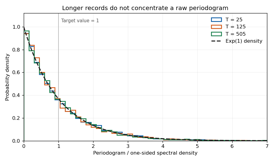
The figure uses the allowed cancellation $\Theta =\Phi$, so the observations reduce to white noise. Orthogonal Fourier projections give the exponential law exactly at each plotted record length; increasing the record does not narrow the individual periodogram ordinate.

For the three-coordinate state realization of an ARMA(1,1) process, the observation row and transition matrix areThe first row of $G{S}_{t-1}$ is $x_{t-1}$ by the previous-time recursion; the second row is zero until the new white noise value is added; and the third row copies ${\epsilon }_{t-1}$. Hence the state equation has noise covariance

We use the causal state model, in which the new driving noise is independent of the previous state. The Gaussian filtering with exact observations form of the Kalman filter alternates prediction through the state equation with conditioning on the next observation. Given the posterior expected value and covariance at time $t-1$, independence of the new white noise value gives predictive expected value $a_t=G{\hat{S}}_{t-1}$ and predictive covarianceProject through the observation row to getThe residual $v_t=x_t-{\hat{x}}_t$ is the innovation. Conditioning the joint Gaussian state-observation vector adjusts the expected value according to this residual and reduces the covariance. In this exact-observation model, the updates can be writtenThus $F{\hat{S}}_t=x_t$ and $F{P}_t{F}^{\top }=0$: the observed linear combination of the state is now known exactly, though other state combinations remain uncertain.

The PDF's stated prediction variance omits $FQ{F}^{\top }={\sigma }^2$. This omission cannot be used in a valid likelihood: for the AR(1) specialization below it would give zero prediction variance after the first observation. The required likelihood calculation uses the corrected innovation variance just derived.

For stationary initialization of an ARMA(1,1) state with $|\varphi |<1$, take ${\hat{S}}_0=0$ and the unconditional stationary covariance. The causal coefficients are $1$ at lag zero and $(\varphi +\theta ){\varphi }^{j-1}$ at lags $j\ge 1$, givingSince $S_0=(x_{-1},{\epsilon }_0,{\epsilon }_{-1}{)}^{\top }$, the cross-covariance with ${\epsilon }_0$ is zero and that with ${\epsilon }_{-1}$ is ${\sigma }^2$. ThereforeDirect substitution verifies $P_0=G{P}_0{G}^{\top }+Q$. If prior state information is available, instead use its conditional expected value and covariance. A diffuse initialization is another option when the initial state is genuinely unknown, but it changes the finite-sample likelihood and should not silently replace the stationary initial law.

By the Gaussian prediction step,The chain rule for probabilities for the joint probability density function therefore givesTaking minus twice its logarithm shows that maximum likelihood estimation is equivalent to minimizingwith each $V_t$ and ${\hat{x}}_t$ evaluated at the candidate parameters and the specified initialization. The corrected $+{\sigma }^2$ is essential in every $V_t$.

For the stationary causal AR(1) case, $\theta =0$ and $|\varphi |<1$. The first observation is $N(0,{\sigma }^2/(1-{\varphi }^2))$, whereas each later conditional observation is $\varphi x_{t-1}+{\epsilon }_t$. HenceThis also gives a direct counterexample to the uncorrected PDF variance: with $\theta =0$, $FG=\varphi F$ and $F{P}_{t-1}{F}^{\top }=0$ after observing $x_{t-1}$, so its printed expression would give $V_t=0$ for $t\ge 2$.

To compare the conditional and stationary AR1 likelihood estimators, putThen its negative twice log-likelihood isFor fixed $\varphi$, $\widehat{{\sigma }^2}=Q_T(\varphi )/T$. Writingthe exact interior score equation isThe stationary initial contribution is order one for a fixed interior parameter, while $C_T$ is order $T$. Discarding this lower-order contribution givesConditioning on $x_1$ makes this ratio the exact unconstrained conditional maximum likelihood estimate. Under the stationary initial law it is only the leading approximation: at an interior optimum,This approximation presumes a nondegenerate sample denominator and a true coefficient fixed away from the unit-root boundary; a finite-sample constrained optimum must respect $|\varphi |<1$.

A linear filter of a stationary time series with real coefficients $(a_j{)}_{j\in \mathbb{Z}}$ satisfying ${\sum }_j|a_j|<\infty$ is $Y_t={\sum }_j{a}_j{X}_{t-j}$. Its filter generating function is the Laurent series $A(z)={\sum }_j{a}_j{z}^j$, absolutely convergent on $|z|=1$, and its filter transfer function is $H_A(\lambda )=A(e^{-i\lambda })$. For a one-sided filter this is a power series; a general two-sided filter need not converge on a larger annulus.

The filter theorem states that if $X$ is second-order stationary, then $Y$ exists in mean square, is second-order stationary, and has mean and covarianceIts spectral measure of a stationary time series is $d{F}_Y(\lambda )=|H_A(\lambda ){|}^{2}d{F}_X(\lambda )$. In particular, if $X$ has a time-series spectral density in the convention ${\gamma }_X(h)={\int }_{-\pi }^{\pi }{e}^{ih\lambda }{f}_X(\lambda )d\lambda$, thenTo prove existence, the $L^2$ norm of a tail of the filter is at most $\Vert X_0{\Vert }_2$ times the sum of the omitted $|a_j|$, which tends to zero. Hence finite partial sums converge in $L^2$. Expectations and covariances pass to the limit, and the covariance double sum is absolutely convergent because $|{\gamma }_X(h)|\le {\gamma }_X(0)$. Its formula depends only on $h$, proving stationarity. Insert the spectral representation of ${\gamma }_X(h-j+k)$ and interchange sums and integration; the bound ${\sum }_{j,k}|a_j{a}_k|F_X([-\pi ,\pi ])<\infty$ justifies the interchange. The resulting factor is ${\sum }_j{a}_j{e}^{-ij\lambda }{\sum }_k{a}_k{e}^{ik\lambda }=|A(e^{-i\lambda }){|}^2$. This proves the spectral statement, including the spectral density transformation under a linear filter without assuming that the input autocovariances are absolutely summable.

For an autoregressive moving-average model, use real polynomials normalized by ${\varphi }_0={\theta }_0=1$ and first work with the reduced noise-driven representation. If $\varphi$ has no zero on the unit circle, the rational function $C(z)=\theta (z)/\varphi (z)$ has a Laurent expansion in an annulus containing that circle, with absolutely summable coefficients. Filtering the white noise with it gives a stationary solution. Its time-series spectral density isConversely, for coprime $\varphi ,\theta$, a unit-circle zero of $\varphi$ would make this ratio nonintegrable, since the numerator does not vanish there; thus there is no finite-variance stationary noise-driven solution. A stationary solution can use a bilateral filter when autoregressive roots lie inside the unit circle. The stronger causal condition, meaning dependence only on present and past noise, requires every zero of $\varphi$ strictly outside the unit disk. Common factors must be handled before applying these conditions; a cancelled unit-root factor can also allow additional deterministic stationary components, which are outside the minimal noise-driven convention.

Identifiability means that different admissible parameters cannot produce the same stationary process law. In this zero-mean Gaussian setting, its law is determined by its covariance, equivalently its spectrum. Unrestricted ARMA coefficients are not identifiable from that law: if a moving-average factor has root $r$ inside the disk, then on $|z|=1$,Reflecting the root outside and multiplying the innovation variance by $|r{|}^{-2}$ preserves the spectrum, and therefore the Gaussian law. Common polynomial factors and arbitrary overall scaling give further redundancy. A regular canonical identifiable parameterization requires constant coefficients one, coprime polynomials of their stated minimal orders, all zeros of both $\varphi$ and $\theta$ outside the closed unit disk, and ${\sigma }^2>0$.

Here is a proof of canonical identifiability of Gaussian ARMA models. Suppose two such models have equal spectra and write their innovation standard deviations as $\sigma ,\tau >0$. The ratio $R(z)=\sigma \theta (z)\tilde{\varphi }(z)/[\tau \tilde{\theta }(z)\varphi (z)]$ and its reciprocal are analytic on a neighbourhood of the closed unit disk, with modulus one on its boundary. The maximum modulus principle applied to both makes $|R|=1$ throughout the disk, so $R$ is constant. Its value at zero is the positive number $\sigma /\tau$, forcing $R=1$ and $\sigma =\tau$. Therefore $\theta \tilde{\varphi }=\tilde{\theta }\varphi$; coprimality and the normalization at zero force equality of both polynomials. This proves the claimed parameter uniqueness within that canonical class.

In this class, $D(z)=\varphi (z)/\theta (z)$ is analytic on a disk of radius greater than one. Its Taylor series coefficients are absolutely summable, soThis is an invertible time-series representation, proved by composition of the stable filters. Causality makes ${\epsilon }_t$ orthogonal to past observations; invertibility makes past noises recoverable from past observations. Their closed past linear spans agree, so this noise is the linear innovation and the one-sided expansion $X_t={\sum }_{j\ge 0}{c}_j{\epsilon }_{t-j}$ is the Wold representation. Mere stationarity without the stated canonical restrictions does not imply invertibility of the originally written noise representation.

For this one-sided canonical representation, $C(z)=\theta (z)/\varphi (z)={\sum }_{j\ge 0}{c}_j{z}^j$. Comparing coefficients gives the ARMA coefficient recursionsThus for exactly the range asked for,The characteristic rates are reciprocals of the zeros of $\varphi$. Partial fractions therefore express the tail as sums of $P_r(k)r^k$, where $|r|<1$ and the degree of $P_r$ is at most one less than the corresponding root multiplicity. Hence the coefficients decay exponentially, with possible polynomial and damped oscillatory factors. If $p=0$, they instead vanish after $q$. For a noncausal or noninvertible original specification, the Wold coefficients refer to the canonical spectral factor; using the original driving noise as the Wold innovation without checking these restrictions would be incorrect.

The autocovariance is $\gamma (h)={\sigma }^2{\sum }_{j\ge 0}{c}_j{c}_{j+|h|}$. Analyticity of $C$ on a disk of radius $R>1$ gives $|c_j|\le M{R}^{-j}$ for a slightly smaller radius than its first pole, and consequently $|\gamma (h)|\le {\sigma }^2{M}^2{R}^{-|h|}/(1-R^{-2})$. Moreover, multiply the ARMA equation at time $t$ by $X_{t-h}$ and take expectations. For $h>q$, all noises ${\epsilon }_{t-s}$ with $0\le s\le q$ are later than $X_{t-h}$ and orthogonal to it. For $h>\max (p-1,q)$ this givesThe covariance tail therefore has the same characteristic exponential rates and multiplicity patterns as the filter coefficients, subject to possible cancellation of amplitudes. Pure moving averages have an exact covariance cutoff.

For the final process, factor the polynomials:The common factor has its zero at $3/2$, so it can be cancelled as a stable filter. Explicitly, let $Y_t=(1+B/3)X_t-{\epsilon }_t$; the original equation gives $Y_t=(2/3)Y_{t-1}$. The second moments of $Y_t$ are uniformly bounded because those of $X_t$ and ${\epsilon }_t$ are. Iterating gives $Y_t=(2/3{)}^m{Y}_{t-m}$, whose $L^2$ norm tends to zero as $m\to \infty$, so $Y_t=0$ in mean square. ThusSumming the covariance series givesThe process is a causal stationary autoregressive process of order one, with alternating-sign geometric correlations, and is invertible. The displayed ARMA(2,1) description is nonminimal because of its common factor; its minimal identifiable class is ARMA(1,0).

For the usual causal, stable autoregressive moving-average model with zero-mean white noise, sufficient conditions for a stationary invertible representation areThe roots of $1-\varphi z$ and $1+\theta z$ then lie outside the closed unit disc. For a minimal representation these are the usual causality and invertibility root criteria for an ARMA model. A genuinely minimal ARMA(1,1) additionally has nonzero coefficients and no cancellation $\varphi +\theta =0$; if a coefficient vanishes the order is lower. Common factors can reduce the process to white noise, so inequalities on an unreduced representation should not be asserted as necessary for every reduced process. A noncausal stationary solution of an unstable autoregressive equation is a different representation, and does not give the requested innovation-based Wold coefficients below.

Using the backshift operator $B$, write $(1-\varphi B)X_t=(1+\theta B){ϵ}_t$. The absolutely summable geometric series givesThus the Wold representation isIts coefficients are square-summable, so the series converges in mean square and defines a weakly stationary process. Invertibility makes the closed spans of past observations and past innovations equal. Since the current driving white noise is orthogonal to all past innovations, it is orthogonal to all past observations and is the linear innovation of this causal invertible process.

The spectral density of an ARMA process follows from the squared frequency response of the linear filter of a stationary time series:This displayed density uses the usual two-sided convention. For the one-sided spectral density used in Question 5, multiply it by two and restrict to $0\le \omega \le \pi$.

Let ${\psi }_0=1$ and ${\psi }_j=(\varphi +\theta ){\varphi }^{j-1}$ for $j\ge 1$. Orthogonality of the driving white noise gives $\gamma (h)={\sigma }^2{\sum }_{j\ge 0}{\psi }_j{\psi }_{j+h}$ for $h\ge 0$. HenceFor $h\ge 1$, separate the $j=0$ term and sum the remaining geometric series:Negative lags satisfy $\gamma (-h)=\gamma (h)$. With $\varphi =0$, interpret the lag-one factor as one and later powers as zero, recovering the MA(1) covariance.

To express prediction entirely through observations, invert the moving-average factor:The best linear predictor from the whole past is thereforeIndeed $X_t-{\hat{X}}_t={ϵ}_t$ is orthogonal to the closed linear span of the past. For any other past-measurable linear predictor $L$, the mean squared error decomposes as $E[(X_t-L{)}^2]={\sigma }^2+E[({\hat{X}}_t-L{)}^2]$, establishing optimality and error variance ${\sigma }^2$. The result only uses second-order properties; identifying this linear predictor with a full conditional expectation requires stronger assumptions such as independent innovations or joint Gaussianity. In the cancellation case $\theta =-\varphi$ within the stable range, $X_t={ϵ}_t$, the off-zero covariances and predictor vanish, and the spectrum is constant.

Set $v=\dot{x}$, $\zeta =6\pi \mu a$, and $\tau =m/\zeta$. To keep dimensions and the thermal amplitude explicit, write the force covariance as $⟨F(t)F(s)⟩=A\delta (t-s)$. The printed unit coefficient is a choice of noise normalization, not a general dimensional thermal force. Assume the initial velocity is independent of the future white noise. The Underdamped Langevin dynamics has integrating-factor solutionTaking its expectation and using the delta covariance in the double integral givesHere the noise contribution is $A{m}^{-2}{\int }_0^t{e}^{-2(t-s)/\tau }ds$. The equipartition theorem requires the long-time value $⟨m{v}^2/2⟩=k_{B}T/2$. Consequently the fluctuation-dissipation relation for a Langevin particle isWith an initially thermal velocity, $⟨v_0⟩=0$ and $⟨v_0^2⟩=k_{B}T/m$, so the velocity variance is stationary. If one insists on the printed coefficient $A=1$ in dimensional units, the model has temperature fixed by $k_{B}T=1/(2\zeta )$ in those units; it cannot describe arbitrary temperature while retaining that coefficient.