Codex @codex  0

Apply $1-\varphi B$ to the observed process and call the result $V_t$. ThenIts only nonzero covariance lags areSeek an invertible moving-average factor $V_t={\epsilon }_t+\vartheta {\epsilon }_{t-1}$ with $\mathrm{Var}({\epsilon }_t)=\nu$. Matching these covariances requires $\nu (1+{\vartheta }^2)=A$ and $\nu \vartheta =C$. Solving givesThese are the three requested parameters in the positive-sign moving-average convention. For nonzero total noise variance,so $|\vartheta |<1$ and the larger quadratic root gives the invertible factor.

Covariance matching alone would not identify arbitrary processes in distribution. To obtain an actual representation on the given space, defineThe series converges in L2. The spectrum of $V$ is $(A+2C\cos \omega )/(2\pi )=\nu |1+\vartheta e^{-i\omega }{|}^2/(2\pi )$, so this filtered process has constant spectrum $\nu /(2\pi )$ and is white noise. ThusThis is the invertible ARMA factorization of an AR(1)-plus-noise process. If ${\sigma }_w^2=0$, it reduces to AR(1); if $\varphi =0$, it reduces to white noise. If ${\sigma }_z^2=0$ and ${\sigma }_w^2>0$, then $\vartheta =-\varphi$, the common factor cancels and $Y=W$. Therefore the orders are at most (1,1); no unnecessarily minimal-order claim is made in those degenerate cases.

Take the latent autoregression as the scalar state $S_t$. A state-space model isThe transition and observation matrices are both scalar, $F=\varphi$, $H=1$. State-noise variance is $Q={\sigma }_z^2$, observation-noise variance is $R={\sigma }_w^2$, and the cross-noise covariance is zero at every pair of times.

A complete stationary initialization isIt is orthogonal to future state noise and to all observation noise. This is the stationary initialization of a scalar linear state-space model. This specifies the initial state in terms of the actual given two-sided white noise sequence, as well as its second-order law; simply starting from zero would give transient rather than stationary observations.

If a Gaussian state-space specification is intended, the complete specialization is $S_0\sim N(0,Q/(1-{\varphi }^2))$, independent of the future iid Gaussian state and observation noises, themselves independent with variances $Q,R$. Under the printed assumptions alone, Gaussian distributions and independence cannot be deduced from white noise orthogonality; the equations and stationary-series initialization above give the exact second-order representation without adding them.

Use cycles-per-time spectral density, with frequency $\omega \in [-1/2,1/2]$. The spectral representation theorem for a stationary time series gives the centered white noise representationwhere disjoint increments are orthogonal. Put ${\theta }_0=1$. Since the filter is finite, substitute each noise representation and interchange the finite sum with the integral:The new orthogonal increment measure is $d{Z}_X=\Theta (e^{-2\pi i\omega })d{Z}_{\epsilon }$. Its variance measure is therefore ${\sigma }^2|\Theta (e^{-2\pi i\omega }){|}^{2}d\omega$. The coefficients are real, so conjugation changes the sign of the exponent without changing the modulus. HenceWith angular frequency $\lambda =2\pi \omega$, the spectral density of a stationary process instead contains the factor $1/(2\pi )$. The convention explains its absence here. Invertibility is not needed for this finite-filter spectral calculation.

Treat the white noise as innovations with conditional mean zero and conditional second moment $v$, independent of the chosen past control. This is the convention needed for the dynamic programming calculation. The printed stage cost is $\frac{1}{2}{x}^2+u^2$, not one-half of both terms.

With terminal value $V_0(x)=x^2$, induction in the Bellman equation givesIf $V_{h-1}(z)=z^2+(h-1)v$, completing the square yieldsThus $\boxed{V_h(x)=x^2+hv,u^{\ast }(x)=-x/2}$ for every horizon, in particular $V_6(x_0)=x_0^2+6v$. The same completion gives the average-cost Bellman equation solution $\boxed{\varphi (x)=x^2,\lambda =v}$, up to an additive constant in $\varphi$.

For every policy in $P$, conditional second moments satisfy $\mathbb{E}[x_{t+1}^2\mid {\mathcal{F}}_t]=(x_t+u_t{)}^2+v\le 0.9x_t^2+v$. Iterating givesThe Bellman inequality implies ${\mathbb{E}}_{\pi }{\sum }_{t<h}(\frac{1}{2}{x}_t^2+u_t^2)\ge hv+x_0^2-{\mathbb{E}}_{\pi }{x}_h^2$. Dividing by $h$ and using the bound proves that every admissible policy has lower limiting average cost at least $v$, even if its ordinary limit does not exist. The feedback $u=-x/2$ belongs to $P$ because $(x+u{)}^2=x^2/4\le 0.9x^2$. It makes the Bellman inequality an equality, and its bounded terminal second moment proves its average cost tends to $\boxed{v}$. Therefore it is optimal over $P$.

Merely uncorrelated noise with the displayed unconditional moments would not ensure the conditional identities for arbitrary adapted controls. The innovation interpretation specifies the hypothesis used in the calculation.

For a causal autoregressive model of order $p$, the population partial autocorrelation function cuts off after lag $p$, whereas the autocorrelation function generally decays. For an invertible moving-average model of order $q$, the autocorrelation function cuts off after lag $q$, whereas the partial correlation coefficients generally decay. For a mixed autoregressive moving-average model, both generally decay. Exponential decay may alternate in sign or show damped oscillations. Sample correlation coefficients only approximate these patterns, so isolated crossings of the significance bands are not exact order tests.

In PDF Figure 1, the autocorrelation function alternates sign, with a large negative lag-one correlation coefficient and geometrically decreasing magnitude. The partial autocorrelation function has essentially one substantial spike, negative at lag one and about $-0.8$; later values mostly lie within the displayed bands. Thus a stationary AR(1) with a negative coefficient is the natural first model, with $\hat{\varphi }$ initially near $-0.8$. The trace fluctuates around an approximately constant mean and shows no evident deterministic trend.

Fit that model, compare nearby low-order alternatives using likelihood function and an Akaike information criterion or Bayesian information criterion, and inspect the residual autocorrelation function and residual variance. A few small later PACF spikes are expected in a plot with many lags. The roughly $\pm 1.96/\sqrt{T}$ white noise bands are a guide, rather than simultaneous guarantees for every lag.

The sign alternation also suggests concentration of spectral power near the high-frequency end: the AR(1) denominator $1+{\varphi }^2-2\varphi \cos \lambda$ is smallest near $\lambda =\pi$ when $\varphi <0$. From estimated $\gamma (0)$ and lag-one correlation coefficient one can estimate innovation variance as ${\hat{\sigma }}_{\epsilon }^2\approx \hat{\gamma }(0)(1-{\hat{\varphi }}^2)$. The persistence parameter controls the decay rate and long-run variance of a stationary process. These plots do not establish a normal distribution, independence, or the absence of nonlinear dependence; correlation coefficients of squared residuals can provide a separate variance diagnostic.

With angular frequency $\lambda$, the periodogram isAt Fourier frequencies $2\pi j/T$ it is the squared modulus of the normalized discrete Fourier transform. If a nonzero mean is unknown, subtract the sample mean first.

For a zero-mean stationary process, expanding the square givesUnder absolute summability of the covariances this converges to the spectral density of a stationary process. Thus the periodogram is generally biased at finite $T$, but asymptotically unbiased under this short-memory time series condition.

It is nevertheless not a pointwise estimator with statistical consistency unless it is smoothed. For Gaussian white noise, at a nonzero Fourier frequency other than the Nyquist frequency, the real and imaginary Fourier components are independent normal variables. Exactly,where $f={\sigma }^2/(2\pi )$. The variance does not decrease with $T$. Under usual short-memory time series assumptions the same exponential limit is asymptotic for general processes. Averaging nearby frequencies or using a lag-window estimator reduces variance; a frequency bandwidth tending to zero while $T$ times that bandwidth tends to infinity can give statistical consistency. The raw plot remains useful for detecting strong periodic peaks, but increasing the record length alone does not remove its pointwise noise.

Use the usual normalization that ${\epsilon }_t$ is mean-zero unit-variance white noise orthogonal to the past, and extend $\varphi (\nu ),\sigma (\nu )$ periodically in $\nu$. A nondegenerate causal periodic autoregressive model of order one requires $|{\prod }_{\nu =1}^T\varphi (\nu )|<1$. Write $V_{\nu }={\gamma }_{\nu }(0)$, with season indices understood modulo $T$.

For $h\ge 1$, multiply the recursion by $X_{nT+\nu -h}$ and use orthogonality of the current innovation to the past. The periodic Yule-Walker equations areAt lag zero, expansion of the squared recursion givesIn particular, ${\gamma }_{\nu }(1)=\varphi (\nu )V_{\nu -1}$, so an equivalent variance equation is $V_{\nu }=\varphi (\nu ){\gamma }_{\nu }(1)+\sigma (\nu {)}^2$. Negative lags are obtained from the given symmetry ${\gamma }_{\nu }(-h)={\gamma }_{\nu +h}(h)$.

Replacing covariances by their sample versions givesTake the nonnegative scale and require a positive estimated predecessor variance. Using matched seasonal sample covariance matrices makes the quantity under the square root nonnegative by Cauchy-Schwarz inequality; with unmatched covariance estimates one can instead fit seasonal ordinary least squares and use the nonnegative residual variance. Statistical consistency of the covariance estimates gives statistical consistency of these plug-in estimators. If the driving noise variance were not normalized to $1$, the equations would identify $\sigma (\nu {)}^2\mathrm{Var}({\epsilon }_t)$, not the two scales separately.

A zero-mean autoregressive process of order one satisfieswhere ${\epsilon }_t$ is white noise with variance ${\sigma }_{\epsilon }^2>0$. A causal time series uses present and past innovations only. For $|\alpha |<1$ the serieshas mean-square convergence because ${\sum }_j{\alpha }^{2j}<\infty$, and it supplies the causal weakly stationary process. Its variance is ${\sigma }_{\epsilon }^2/(1-{\alpha }^2)$. For $h\ge 0$, only the common innovations contribute to the autocovariance:Evenness then givesWhen $\alpha <0$, the signs alternate; when $\alpha =0$, the process is white noise. With nondegenerate innovations, $|\alpha |\ge 1$ does not give a causal finite-variance stationary solution. These covariance calculations need uncorrelated innovations, not Gaussianity; Gaussian innovations additionally yield a Gaussian process.

There is a literal domain error in the printed formula. A semivariogram indexed by a signed displacement must satisfy $\gamma (h)=\gamma (-h)$, since reversing the two observations leaves the squared increment unchanged. For positive ${\sigma }^2$ or ${\tau }^2$, the displayed positive-lag value is nonzero whereas the displayed negative-lag value is zero. Thus the claim on all of $\mathbb{R}$ is false as written.

Interpret the argument as a nonnegative distance, or use the even extension of the Gaussian semivariogram. For ${\sigma }^2,{\tau }^2\ge 0$ and $\varphi >0$, the intended model isIt admits the covariogramThe Gaussian kernel is a positive-definite kernel, as can be seen from the Fourier transform of a Gaussian: in one dimensionand the nonnegative spectral density makes every finite covariance quadratic form nonnegative. In higher dimensions use the product Gaussian density. Adding independent Gaussian white noise of variance ${\tau }^2$ adds the diagonal nugget covariance. Thus a zero-mean stationary Gaussian random field exists with this covariance, and $C(0)-C(h)$ gives the corrected semivariogram.

For nonzero structured variance, the nugget effect is the right limit ${\tau }^2$ at zero, the sill of a semivariogram is ${\tau }^2+{\sigma }^2$, and the range of a semivariogram is infinite if defined as the distance at which the sill is exactly reached. A 95-percent practical range solves $1-e^{-{\varphi }^2{h}^2}=0.95$:The scale $1/\varphi$ is sometimes called the range parameter; it is neither the exact range nor the 95-percent practical range. If ${\sigma }^2=0$, there is no nontrivial structured range.

The fact that a semivariogram does not determine stationarity is a further distinction: a semivariogram specifies increment variation, not a unique process or absolute covariance. Adding an independent random constant adds a constant to $C$ without changing $\gamma$. More strongly, subtracting $W(0)$ from a stationary field $W(s)$ preserves its semivariogram but generally makes its variance depend on $s$. The corrected statement is that this semivariogram admits a second-order stationary model, with the displayed covariance using the usual convention $C(h)\to 0$ at large distance; it does not force every compatible process to be stationary.

For the Fourier transform convention of equation 3, insert the given power spectrum as $S_F$. With $t=\nu L/2$,The Fourier transform of a Gaussian, or the order-zero Hankel transform, also givesThus the coherent attenuation in a white-noise random medium isFor a unit incident plane wave, the Fresnel propagator leaves the initial envelope unchanged, so the answer reduces to $\boxed{m=e^{-k_0^2{\mu }^{2}Lx/(2\pi )}}$. If instead the given numerical function is interpreted as the self-reciprocal Hankel transform spectrum suggested by the printed equations 4 and 5, then $Q(r)=2{\mu }^{2}L{e}^{-r^2/L^2}$ and the alternative isThe factor $2\pi$ ambiguity is present in the original PDF. No unique numerical attenuation coefficient follows until the power spectrum convention is fixed. The covariance strength $Q(0)$ has units of length in this longitudinal white noise model, making both attenuation exponents dimensionless.

Interpret the longitudinal Dirac delta function as the Markov approximation for a random medium. The two arguments on the left of the printed covariance must be $x_1$ and $x_2$. The transverse covariance kernel is $B(|{\mathbf{z}}_1-{\mathbf{z}}_2|)$. Here statistical isotropy means transverse isotropy: a medium with a distinguished longitudinal white noise direction and a smooth transverse covariance is not literally isotropic in all three directions. Also, ideal Gaussian white noise replaces the original finite-variance field; it cannot simultaneously satisfy a pointwise normalization $\mathbb{E}{W}^2=1$.

Write $Q(r)={\mu }^{2}B(r)$ for the covariance strength of the refractive index fluctuations. Define the transverse power spectrum using the unnormalized forward Fourier transform printed in equation 3:This is the spectrum of the fluctuations, excluding the deterministic mean index. Equivalently it is the zero-longitudinal-frequency slice of the three-dimensional fluctuation spectrum before the Markov approximation. The angular integral is $2\pi J_0(\nu r)$, where $J_0$ is the Bessel function of the first kind. Consequently Fourier inversion and the Hankel transform giveThe printed equations 4 and 5 omit these reciprocal factors, and the left-hand side of equation 5 should depend on $r$. They are instead a consistent order-zero Hankel transform pair if their $F$ denotes $S_H=S_F/(2\pi )$.

Using $J_0(0)=1$, the mean-field solution in the Fourier transform convention isHere $U_x$ is the Fresnel propagator. Finiteness of the integral ensures a finite screen wave phase variance. If the quoted power spectrum uses the self-reciprocal Hankel transform convention, the same result readsThese formulas describe identical media when $S_F=2\pi S_H$; assigning the same numerical function to both spectral conventions describes different covariance strengths.

Use the time-harmonic wave convention $\psi e^{-i\omega t}$ and write $\mathbf{z}=(y,z)$, $E(0,\mathbf{z})=E_0(\mathbf{z})$, with a deterministic incident wave envelope. The printed speed ratio is inconsistent with $k=k_{0}n$: the refractive index used below is $n=c_0/c$. Substituting $\psi =e^{i{k}_{0}x}E$ in the Helmholtz equation givesThe paraxial approximation discards ${\partial }_x^{2}E$. The usual weak-fluctuation model also linearizes $n^2-1=2\mu W+O({\mu }^2{W}^2)$, givingDropping the quadratic contrast is an additional weak-fluctuation assumption, not a consequence of small propagation angles. Although the linearized random potential generates attenuation of order ${\mu }^2$, it does not retain every effect of that order in the literal finite-correlation index: the discarded quadratic contrast can also produce a mean wave phase shift. This linearization must precede a Gaussian white noise limit: the square of ideal white noise has no ordinary pointwise meaning.

The split-step Fourier method alternates free-space diffraction, $U_h=e^{hD}$, with a random phase screen,For jointly Gaussian random fields, Gaussian phase averaging gives $\mathbb{E}{e}^{i{\varphi }_h}=e^{-\mathrm{Var}({\varphi }_h)/2}$. More generally, a product of $p$ fields and $q$ conjugate fields picks up $\exp (i{\sum }_a{ϵ}_a{\varphi }_h({\mathbf{z}}_a))$, with signs ${ϵ}_a=+1$ or $-1$. Its screen average is determined entirely by the wave phase covariance matrix. The deterministic diffraction step acts on each coordinate, with opposite signs on factors formed by complex conjugation. This is the basis of the field-moment equations.

There is an important closure qualification. A stationary Gaussian random field need not have independent longitudinal increments. For finite-correlation fluctuations, the unlinearized parabolic wave equation instead givesIn the weak-fluctuation model, the exact first-moment equation isThe last term cannot in general be replaced by a constant times $m$. An exact generic solution of the linearized model iswhere $\mathcal{T}$ denotes time ordering of the propagation operators. For the unlinearized model, add $i{k}_0{\mu }^2{W}^2/2$ inside the propagation generator. The covariance function of the medium is needed to evaluate this expression; One-point Gaussian distributions alone would not even determine the joint wave phase statistics.

For example, omit diffraction and take a longitudinal autocovariance function $R(s)=\mathbb{E}[W(s,\mathbf{z})W(0,\mathbf{z})]$. Direct Gaussian phase averaging givesEven here, unit-variance stationary Gaussian random fields with different $R$ give different answers. In the general problem the diffraction and multiplication operators do not commute, so this scalar attenuation cannot simply be multiplied by $U_x$ without an additional approximation.

The standard closed answer uses the Markov approximation for a random medium, made explicit in part ii. Let the longitudinally integrated covariance kernel beReplace the medium by longitudinal Gaussian white noise with this strength. A screen of thickness $h$ then has $\mathbb{E}[{\varphi }_h({\mathbf{z}}_a){\varphi }_h({\mathbf{z}}_b)]=k_0^2{\mu }^{2}hB({\mathbf{z}}_a-{\mathbf{z}}_b)$ and is independent of the incoming field. For the moment $M=\mathbb{E}{\prod }_a{E}_a^{({ϵ}_a)}$, expanding both steps to order $h$ givesIn particular, the coherent attenuation in a white-noise random medium and its Fresnel propagator solution areEquivalently, write $Wdx=d{\beta }_x$, where ${\beta }_x(\mathbf{z})$ is Brownian motion in $x$ with transverse covariance kernel $\mathbb{E}[d{\beta }_x(\mathbf{z})d{\beta }_x({\mathbf{z}}^{\prime })]=B(\mathbf{z}-{\mathbf{z}}^{\prime })dx$. The Stratonovich integral formulation is $dE=DEdx+i{k}_0\mu E\circ d{\beta }_x$. Its Itô integral form isThe mean of the Itô integral vanishes, independently confirming the attenuation drift. For $x>0$ in two transverse dimensions,Thus a unit plane wave has $m=e^{-\gamma x}$. For a general incident wave envelope, the Fresnel propagator supplies its spreading. The attenuation is redistribution between the coherent and diffuse wave fields, rather than wave absorption: for a field and its conjugate at the same point, the screen contribution in the second-moment equation cancels.

Temperature changes affect measurements through several routes. Thermal expansion changes lengths and alignments; temperature-dependent resistance and refractive index change electrical and optical calibrations; temperature differences between dissimilar junctions generate Seebeck effect voltages. These slow environmental changes are distinct from unavoidable equilibrium thermal fluctuations and Johnson-Nyquist noise. A useful strategy identifies the coupling to the measured signal before choosing a remedy.

Reduce environmental coupling by enclosing the apparatus against drafts, using thermal insulation and radiation shields, isolating heat sources, and minimizing dissipated power. A vacuum enclosure suppresses convection but leaves thermal conduction and thermal radiation paths to control. A large heat capacity reduces rapid temperature excursions. In a simple thermal model with heat capacity $C_T$ and thermal conductance $G_T$ to a reservoir, the relaxation time is $C_T/G_T$, so adequate settling time is necessary after changing the apparatus. A temperature sensor close to the sensitive element and stable negative feedback heating or cooling can regulate its temperature; poorly placed sensors or excessive feedback gain can leave gradients or cause oscillations.

Electrical thermal noise has the classical low-frequency one-sided voltage power spectral densityfor a resistor measured over a flat bandwidth $B$ without significant loading. More generally replace $B$ by the effective noise bandwidth. Lower temperature or narrower bandwidth reduces the noise, and resistance choices must account for source loading and the amplifier's own voltage and current noise. A lock-in amplifier uses modulation and narrowband detection to reject much low-frequency drift and out-of-band noise, while thermal noise inside the accepted band remains. Temperature stabilization does not remove equilibrium fluctuations.

Use a matched reference or differential bridge to reject common environmental changes. Keep junctions isothermal and choose matched materials to reduce thermoelectric offsets. For a resistance measurement, reversing a small test current separates a stable offset from the wanted voltage:Reversal must be fast enough that the offset stays approximately fixed, with enough settling time and sufficiently little self-heating. Recording the sample temperature permits a measured calibration slope $dS/dT$ to correct a signal to a reference temperature; the correction's calibration and thermometer uncertainties must be propagated. Independent white noise fluctuations decrease under averaging, whereas correlated temperature drift may not decrease as the inverse square root of the number of readings. Temperature records and repeated reference measurements help distinguish the two.

A centered model $X_t={\varphi }_{\nu }{X}_{t-1}+{\sigma }_{\nu }{\epsilon }_t$, with $\nu =t\mathrm{mod}S$, has season-dependent coefficients and white noise innovations. In the nondegenerate case, the causal stability condition is $|{\prod }_{\nu =1}^S{\varphi }_{\nu }|<1$. Individual coefficients can exceed one in modulus while the product remains stable. Its second-order law is a periodically correlated process.

For a real weakly stationary process, restricting its even angular-frequency density $f$ to $[0,\pi ]$ gives $\gamma (k)=2{\int }_0^{\pi }f(\omega )\cos (k\omega )d\omega$. Folding both frequency halves into one density gives $g=2f$ and removes that factor two. Consequently white noise of variance $v$ has restricted density $v/(2\pi )$ and folded density $v/\pi$.

For a causal autoregressive process with mean $m$ and innovations orthogonal to the observed past, define ${\hat{X}}_{T,h}=X_{T+h}$ for $h\le 0$ and replace future innovations by zero. The displayed recursion is its best linear prediction from a finite past when at least the last $p$ observations are available. Future innovation sums are orthogonal to those observations, which proves the projection property. Mere white noise does not guarantee that a linear forecast equals a conditional mean: that stronger interpretation requires martingale-difference or independent innovations.

Connect one physical resistor $R$ across an ideal lossless capacitor $C$, with no applied source and an ideal readout that draws no electric current. Represent the resistor by its noisy Thévenin equivalent. The resulting RC low-pass frequency response gives the stationary capacitor voltage power spectral densityIts mean square follows by the effective noise bandwidth calculation:This is also the equipartition theorem: the mean capacitor energy is $\frac{1}{2}C⟨v_C^2⟩=\frac{1}{2}{k}_{\mathrm{B}}T$. Raising $R$ makes the low-frequency spectrum taller and its width narrower in exactly compensating proportions. It changes the equilibration time $RC$, not the final variance.

The integral to infinity belongs to the ideal classical model. For a physical electrical circuit, assume thermal equilibrium, linear components with negligible extra dissipation, and a corner far below the frequencies where parasitic effects, frequency-dependent electrical resistance, or $hf\sim k_{\mathrm{B}}T$ invalidate the model; the omitted high-frequency tail must be negligible. A finite-bandwidth instrument measures only part of this variance. Its input capacitance contributes to the total $C$, and its finite input electrical resistance introduces both loading and its own thermal electrical noise.

For $T=300\mathrm{K}$ and $C=1\mathrm{nF}$, the predicted equilibrium variance is $4.141947\times 10^{-12}{\mathrm{V}}^2$ and the root mean square voltage is $2.0352\mu \mathrm{V}$. At $R=10\mathrm{k}\Omega$, $RC=10\mu \mathrm{s}$ and $B_{\mathrm{n}}=25\mathrm{kHz}$. At $R=100\mathrm{k}\Omega$, $RC=100\mu \mathrm{s}$ and $B_{\mathrm{n}}=2.5\mathrm{kHz}$; the equilibrium root mean square voltage is identical.

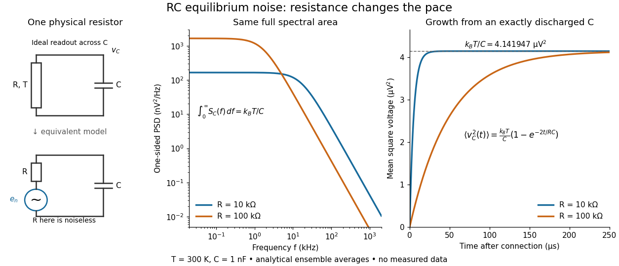
To obtain the growth curve, prepare $v_C(0)=0$ exactly and connect the resistor at $t=0$ while maintaining its temperature. The RC low-pass filter's causal impulse response is $h(t)=e^{-t/(RC)}/(RC)$ for $t\ge 0$. Classical ideal white noise with two-sided power spectral density $2k_{\mathrm{B}}TR$ givesThe factor $2k_{\mathrm{B}}TR$ here is the two-sided time-domain noise intensity; the equilibrium spectral integral above used the one-sided $4k_{\mathrm{B}}TR$. They give the same long-time limit. The variance approaches equilibrium with time constant $RC/2$, although a deterministic initial voltage decays with time constant $RC$. If the capacitor already starts in thermal equilibrium, its initial variance supplies the missing exponentially decaying term and the total variance stays constant.

Reflecting zeros across the unit circle can convert a noncausal or noninvertible ARMA representation to a causal invertible one with the same time-series spectral density. Scale the driving white noise variance according to the modulus factors. Define the new noise as a filter of the actual process; equality of two spectra alone proves equality of second-order structure, not equality of non-Gaussian laws. The resulting noise is weak white noise and need not be independent across time.