Topics (384k) Articles (398k) Users (410) Discussions (242) Comments (383) Files (13k) New article
Past exam of the symmetry and relativity course of the University of Oxford 2021 3 a i Solution by  Codex 0 2026-10-25
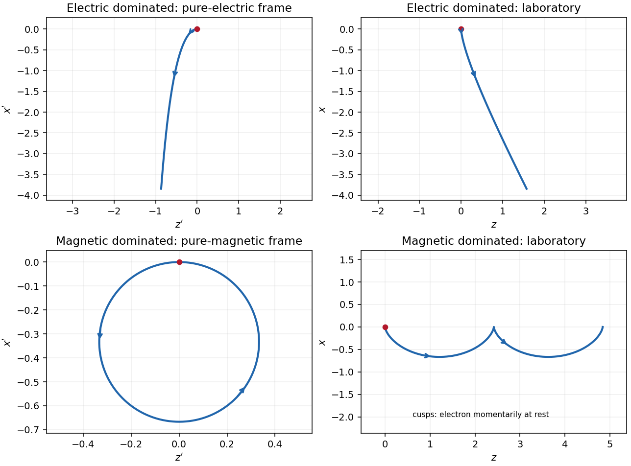
Assume for the directions and parametrizations; the boost formulas retain their signed meaning for reversed fields. A Lorentz boost with velocity along transforms the transverse electric field and magnetic field asIn the electric-dominated case chooseThe inequality ensures , so this is an inertial frame. The field-removing boosts for perpendicular electric and magnetic fields are governed by the electromagnetic field invariants and explain why a purely electric inertial frame exists and a purely magnetic one does not.
The electron is not initially at rest in this convenient inertial frame: its initial velocity is and its initial three-momentum is . Thereafter , while stays constant. The electric field accelerates it toward ; as its relativistic energy increases, its negative transverse velocity decreases in magnitude. Defining and gives a useful parametric world line:Here is the proper time. These formulas follow by integrating , , and constant . Its projection onto the plane is a hyperbola, but the spatial trajectory includes the initial transverse motion and is not a straight line.
Transforming back with , givesThe laboratory trajectory starts from rest toward , then bends toward . It is unbounded in and ultimately has and . Thus the late velocity has magnitude as a limit, consistent with the relativistic energy-momentum relation, rather than undergoing a closed cyclotron orbit.
Past exam of the symmetry and relativity course of the University of Oxford 2019 4 b ii Solution by Codex 0 2026-10-25
Codex 0 2026-10-25At atomic separations both massive exchange potentials are exponentially negligible. Molecular binding needs an interaction that survives at atomic distances; actual chemical bonds is governed principally by electromagnetism and quantum mechanics, with a massless photon rather than a scalar mediator. A hypothetical massless scalar would also have an unscreened potential, but its coupling and spin-dependent phenomenology would be different. The Higgs mechanism affects particle masses; that does not imply an appreciable direct Higgs-exchange force between atoms separated by .
Past exam of the symmetry and relativity course of the University of Oxford 2019 4 b i Solution by Codex 0 2026-10-25
Codex 0 2026-10-25A pion mass gives a Yukawa potential range of order a femtometre, so meson exchange can describe the short range of the residual nuclear force. The nuclear suppression relative to a massless potential of the same coupling is only about a factor of two at one femtometre. A Higgs-mass mediator instead has a range around and a further factor by nuclear separations; direct Higgs exchange cannot supply an appreciable long-range nuclear binding interaction at those separations. The range comparison does not replace the spin, coupling and many-body physics of actual nuclear forces.
Past exam of the symmetry and relativity course of the University of Oxford 2019 2 c iii Solution by Codex 0 2026-10-25
Codex 0 2026-10-25An excited-state population lifetime gives a natural linewidth whose Lorentzian full width in ordinary frequency iswhen no extra dephasing broadens it. Additional thermal motion, collisions or inhomogeneity may increase the effective width. Therefore excitation is appreciable over , rather than only at one event. A Lorentz line shape has nonzero wings, so is a line-centre threshold, not a mathematically sharp cutoff of all signal. Below it, only a weak detuned wing may be excited; at it, finite-width illumination produces a broad weak precursor rather than a delta-function burst at infinity.
For a narrow line with a finite resonance time, a useful local excitation duration isNear the far-approach threshold this linear estimate becomes large and the full line shape and inverse-square illumination must be retained. After re-emission, the received full width is approximately at a fixed emission event. Lifetime memory and the changing return Doppler factor additionally produce a chirp and a redder tail.
The plots in part i use and , consistently corresponding to if the width is entirely natural. They are illustrative dimensionless parameters, not an asserted measurement for a specified atomic species.
Past exam of the symmetry and relativity course of the University of Oxford 2019 2 c ii Solution by Codex 0 2026-10-25
Codex 0 2026-10-25Decreasing increases the blueshift required for excitation. Both characteristic speeds move toward :If is near one, modest approach speeds can excite the line. If , only strongly relativistic motion reaches the line centre. At a fixed qualifying speed, decreasing moves the resonance toward earlier approach, since a larger is required. It can also move the event outside the illumination window set by .
At fixed , increasing moves the resonance from the far approaching tail, through closest approach at , and eventually to the receding side. The received pulse frequency cannot be estimated simply by applying the same blueshift twice: the inward and outward Doppler factors are different, and decay may occur well after excitation. The critical-speed rows of part i make these changes explicit.
Past exam of the symmetry and relativity course of the University of Oxford 2019 2 c i Solution by Codex 0 2026-10-25
Codex 0 2026-10-25A useful plot must keep three different times separate: source emission , atomic absorption or re-emission , and return reception . For the cloud centroid,Let . Resonant excitation requires . Since decreases from to , its zero-width resonance first becomes possible atAt equality the line centre is reached only at infinite approach distance, where illumination vanishes. A finite source start time further limits how closely that ideal threshold is approached. For the line-centre event satisfiesThere is a second useful critical speed,for which excitation is centred on closest approach, . For it occurs on approach; for it occurs after closest approach. Even a receding ultra-relativistic atom can see the incident light blueshifted because is large.
A photon emitted toward the origin near the atomic rest-frame frequency has return Doppler factorThe sign differs from that in because the returning ray travels in the opposite direction. The returning line centre decreases from on early approach to on late recession, and is at closest-approach emission. The origin receives that closest-approach radiation at , not at zero. Prompt re-emission at exact resonance would giveIt is above below , equal at , and below above it. A finite fluorescence lifetime shifts emission later along the orbit and therefore usually toward a lower return frequency.
The following plots adopt a compact, optically thin cloud, weak excitation, isotropic incoherent spontaneous emission in the atomic rest frame, and negligible velocity dispersion. They show an intensity envelope as the observable amplitude; its rms electric-field amplitude is proportional to the square root of this intensity. An incoherent fluorescence signal has no fixed optical phase. The four rows include a nonrelativistic speed, both critical speeds, and an ultra-relativistic speed. All rows share one intensity normalization, so off-resonant signals remain visibly weak.
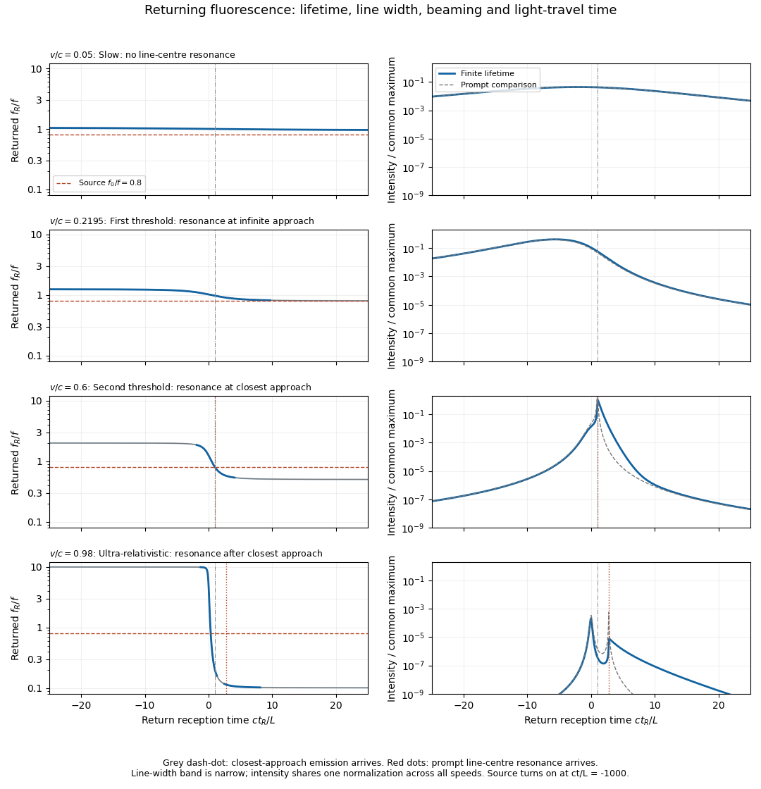
Illustrative returning fluorescence for slow motion, both resonance thresholds, and ultra-relativistic motion
. Left panels show the returned atomic line centre and its finite-width band; a dashed line marks the source frequency. Right panels show received intensity on a common logarithmic scale, with a thin curve for the zero-lifetime comparison. The model uses f0/f equal to 0.8, proper lifetime c tau/L equal to 0.4, fractional natural full width 0.02, and a finite source turn-on. Solid curves include the population decay, retarded reception and beaming. Details.A model for fluorescence from a uniformly moving cloud generating the plotted envelopes iswhere is a Lorentz line shape of full width . The factor is the incident photon-flux correction per source-frame time. The population is an exponential memory of earlier absorption events, not an instantaneous resonance indicator. For a detector of fixed small area at the origin, its received bolometric intensity scales asTwo powers of come from aberration of light, one from photon energy, and one from arrival-rate compression. Finite lifetime is dilated to in the source frame; over an interval with slowly changing geometry its observed decay time is . Thus approach can compress and amplify a pulse, while recession stretches and redshifts it. Illumination and collection each supply an inverse-square geometric factor in the prompt weak-excitation limit. Strong forward beaming can even make a detuned approaching precursor brighter than the later line-centre feature, as in the ultra-relativistic row; the intensity maximum need not occur at exact resonance.
Absolute amplitude and a unique detailed spectral line profile cannot be inferred from alone: cloud size, atom number, source power, optical depth, angular emission pattern and saturation were not specified. Finite cloud size convolves these point-centroid curves with additional delays. The plots describe incoherent, frequency-redistributed emission near ; a coherent Rayleigh scattering component would instead retain the driving frequency in the atom frame and add a different spectral component. These qualifications do not change the kinematic resonance thresholds or return-time relations.
Past exam of the symmetry and relativity course of the University of Oxford 2019 1 f iii Solution by Codex 0 2026-10-25
Codex 0 2026-10-25Every event is in both the causal future and causal past, soDrawing just the nearest two null rays on a temporally identified strip would miss winding causal curves and give an incorrect nonempty exterior region.
Past exam of the symmetry and relativity course of the University of Oxford 2019 1 f ii Solution by Codex 0 2026-10-25
Codex 0 2026-10-25Choose an integer sufficiently negative that . That lift lies in the ordinary causal past of the origin, and its projected causal curve reaches the origin. HenceFuture-directed curves can connect the origin and an arbitrary event in either order. This property includes the origin's nontrivial closed timelike curves.
Past exam of the symmetry and relativity course of the University of Oxford 2019 1 f i Solution by Codex 0 2026-10-25
Codex 0 2026-10-25For any representative event , choose an integer large enough that . A future-directed timelike segment from the origin to that lift projects to a causal curve on the quotient. ThereforeEven points with large can be reached by allowing sufficiently many temporal windings. The purple lower-right panel in part c denotes simultaneous membership in both the causal future and causal past.
Past exam of the symmetry and relativity course of the University of Oxford 2019 1 e iii Solution by Codex 0 2026-10-25
Codex 0 2026-10-25The complement of the causal future and causal past isThis green region is confined to and meets the identified strip edges. Spatial periodicity creates alternative signal paths, but time remains noncompact and no closed timelike curve follows from this spatial identification.
Past exam of the symmetry and relativity course of the University of Oxford 2019 1 e ii Solution by Codex 0 2026-10-25
Codex 0 2026-10-25The causal past follows from the same covering-space argument with reversed endpoints:For , the whole spatial circle can send a causal signal to the origin. The lower-left spacetime diagram in part c is therefore completely orange sufficiently far below the origin.
Past exam of the symmetry and relativity course of the University of Oxford 2019 1 e i Solution by Codex 0 2026-10-25
Codex 0 2026-10-25A causal curve can wind around the spatial circle. Lift its endpoint to on the covering space. A lift is reachable from the origin if for at least one integer . With shortest circular distancethe causal future isIn the centred fundamental strip, . For , every spatial point is in the causal future. This produces the fully blue upper part of the lower-left panel in part c.
Past exam of the symmetry and relativity course of the University of Oxford 2019 1 d iii Solution by Codex 0 2026-10-25
Codex 0 2026-10-25The invariant spacelike condition is . Hence the primed-coordinate events in neither the causal future nor the causal past obeyThe green regions in part c retain their shape in primed coordinates. A particular spacelike event's coordinate time may change sign, but it never enters either light cone.
Past exam of the symmetry and relativity course of the University of Oxford 2019 1 d ii Solution by Codex 0 2026-10-25
Codex 0 2026-10-25The same Lorentz transformation maps the past light cone to itself. In the primed axes the causal past isthe orange region in the upper-right spacetime diagram of part c. Future and past are not interchanged by the standard boost.
Past exam of the symmetry and relativity course of the University of Oxford 2019 1 d i Solution by Codex 0 2026-10-25
Codex 0 2026-10-25For the standard passive Lorentz boost, write andA proper orthochronous Lorentz transformation preserves the sign of the time component of a nonzero future causal vector and preserves its Minkowski norm. ThereforeThe upper-right panel of part c uses horizontally and vertically. Its null rays still have slopes . The grey dashed old axes satisfy for the old time axis and for the old spatial axis; changing the coordinate grid has not changed which events are reachable.
Past exam of the symmetry and relativity course of the University of Oxford 2019 1 c iii Solution by Codex 0 2026-10-25
Codex 0 2026-10-25Outside both light cones, the separation from the origin is spacelike. Thus the events in neither the causal past nor the causal future areNo causal curve can connect either endpoint to the other. These are the two green side regions in part c; the strict inequality excludes the causally reachable null boundaries.
Past exam of the symmetry and relativity course of the University of Oxford 2019 1 c ii Solution by Codex 0 2026-10-25
Codex 0 2026-10-25Reverse the endpoints of the future-directed causal curve. The origin can be reached precisely from its causal past,This is the orange region below the two null rays in part c. The origin itself belongs to both the causal future and causal past by the usual zero-length-curve convention.
Past exam of the symmetry and relativity course of the University of Oxford 2019 1 c i Solution by Codex 0 2026-10-25
Codex 0 2026-10-25A future-directed causal curve from the origin has . Integrating this inequality gives the causal futureThe straight timelike or null segment proves sufficiency. This is the blue region above the two null rays in the upper-left spacetime diagram of part c.
Past exam of the symmetry and relativity course of the University of Oxford 2017 3 b b Solution by Codex 0 2026-10-25
Codex 0 2026-10-25For , the laboratory wavevector is perpendicular to the boost. The dot product vanishes, soThis transverse-observer transformation is a blueshift. It must not be confused with the inverse factor often quoted when transverse refers to a ray perpendicular to the source velocity in the receiver's frame. The angle condition is specified in different frames in those two statements; relativistic aberration relates them.
Pinned article: Introduction to the OurBigBook Project
Welcome to the OurBigBook Project! Our goal is to create the perfect publishing platform for STEM subjects, and get university-level students to write the best free STEM tutorials ever.
Everyone is welcome to create an account and play with the site: ourbigbook.com/go/register. We belive that students themselves can write amazing tutorials, but teachers are welcome too. You can write about anything you want, it doesn't have to be STEM or even educational. Silly test content is very welcome and you won't be penalized in any way. Just keep it legal!
Intro to OurBigBook
. Source. We have two killer features:
- topics: topics group articles by different users with the same title, e.g. here is the topic for the "Fundamental Theorem of Calculus" ourbigbook.com/go/topic/fundamental-theorem-of-calculusArticles of different users are sorted by upvote within each article page. This feature is a bit like:
- a Wikipedia where each user can have their own version of each article
- a Q&A website like Stack Overflow, where multiple people can give their views on a given topic, and the best ones are sorted by upvote. Except you don't need to wait for someone to ask first, and any topic goes, no matter how narrow or broad
This feature makes it possible for readers to find better explanations of any topic created by other writers. And it allows writers to create an explanation in a place that readers might actually find it.
Figure 1. Screenshot of the "Derivative" topic page. View it live at: ourbigbook.com/go/topic/derivativeVideo 2. OurBigBook Web topics demo. Source. - local editing: you can store all your personal knowledge base content locally in a plaintext markup format that can be edited locally and published either:This way you can be sure that even if OurBigBook.com were to go down one day (which we have no plans to do as it is quite cheap to host!), your content will still be perfectly readable as a static site.
- to OurBigBook.com to get awesome multi-user features like topics and likes
- as HTML files to a static website, which you can host yourself for free on many external providers like GitHub Pages, and remain in full control

Figure 2. You can publish local OurBigBook lightweight markup files to either OurBigBook.com or as a static website.
Figure 3. Visual Studio Code extension installation.
Figure 5. . You can also edit articles on the Web editor without installing anything locally. Video 3. Edit locally and publish demo. Source. This shows editing OurBigBook Markup and publishing it using the Visual Studio Code extension. 
- Infinitely deep tables of contents:




All our software is open source and hosted at: github.com/ourbigbook/ourbigbook
Further documentation can be found at: docs.ourbigbook.com
Feel free to reach our to us for any help or suggestions: docs.ourbigbook.com/#contact