For a covering map over a nonempty connected space, the degree of a covering map isthe cardinality of any fibre of a function. To show independence of $x$, choose an evenly covered neighbourhood $U$. Each covering sheet contains exactly one point over every $y\in U$, so $|p^{-1}(y)|$ equals the number of covering sheets over $U$. The fibre of a function cardinality is therefore locally constant. For a fixed cardinal number $\kappa$, the points with that cardinality form an open subset, and their complement is also open. Connectedness forces the value to be constant everywhere.

For a path-connected base there is also an explicit fibre bijection by path lifting: lift a path from $x$ to $y$ starting at each point over $x$ and take its endpoint. The path lifting theorem gives existence and uniqueness; path reversal gives the inverse bijection. The bijection may depend on the path, but the resulting equality of cardinalities does not.

A connected base is needed for one global degree. Without it, use a degree on each connected component on which the cardinality is constant. For example, a covering map of a discrete two-point topological space can have one point over the first point and two over the second. Thus the unqualified printed definition needs the usual connected-base convention, or the explicit assumption that every fibre of a function has the same cardinality.

A covering map is a continuous surjection $p:\tilde{X}\to X$ such that every $x\in X$ has an open neighbourhood $U$ for whichwhere the $U_{\alpha }$ are pairwise disjoint open subsets of $\tilde{X}$. Such a $U$ is an evenly covered neighbourhood, and the sets $U_{\alpha }$ are its covering sheets. The index set may be infinite. The requirement that every sheet map onto all of $U$ is part of the definition.

Let $n=(0,0,1)$ and use the open coverThe cap $V$ is open in $Y$: it equals $Y\cap \{z>1/2\}$ because the attached chord has $z=0$. The cap is homeomorphic to an open disk, and $U\cap V=V\setminus \{n\}$ is a punctured open disk, hence homotopy equivalent to a circle. Both sets and their intersection are path-connected. Choose the base point $b$ in that intersection.

We first calculate ${\pi }_1(U,b)$. A stereographic projection identifies $S^2\setminus \{n\}$ with ${\mathbb{R}}^2$ and sends the two chord endpoints to $(-1,0),(1,0)$. Thus $U$ becomes the Euclidean plane with an extra closed interval attached at those two points. This description is a homeomorphism: gluing the two closed pieces along their endpoints gives exactly the original subspace topology.

The Euclidean plane has a deformation retraction onto $L=[-1,1]\times \{0\}$ while fixing its endpoints. An explicit homotopy isExtend it by the identity map on the extra chord. The pasting lemma for closed subspaces gives a deformation retraction of $U$ onto two distinct closed intervals sharing just their endpoints, a circle. Consequently ${\pi }_1(U,b)\cong \mathbb{Z}$, with the routine base point transport if the retraction moves $b$.

The inclusion-induced group homomorphism ${\pi }_1(U\cap V,b)\to {\pi }_1(U,b)$ is trivial: it factors through $S^2\setminus \{n\}\cong {\mathbb{R}}^2$, which is contractible. Also ${\pi }_1(V,b)=1$. All hypotheses of the Seifert-van Kampen theorem are now checked, and it gives the fundamental group of a sphere with an attached chord:where both maps from the amalgamating infinite cyclic group are trivial. A group generator follows the chord from one endpoint to the other and returns along any path on the sphere, with a connecting path from the chosen base point.

Put $A=T^2\setminus B^2$ and let $E=\partial A=S^1$ denote the attaching circle. The version of the Seifert-van Kampen theorem used here states that if $X=U\cup V$ is an open cover with $U,V,U\cap V$ path-connected and a common base point in $U\cap V$, thenThe expression on the right means the pushout of groups of the two inclusion-induced group homomorphisms; they need not be injective.

Choose a thin collar neighbourhood $C_A$ of $E$ inside $A$, and a thin equatorial band $C_S$ inside $S^2$. For example, before the square's side identifications take $C_A=\{v:1\le |v|<1+ϵ\}$ with $0<ϵ<1/2$, and take $C_S=\{(x,y,z)\in S^2:|z|<ϵ\}$. In the glued topological space setThese are open subsets: their preimages in the two pieces are open and respect the gluing. They cover $X$, and the three deformation retractionsfix $E$. Thus all three spaces are path-connected, and a base point $b\in E$ is preserved.

For completeness, the fundamental group of a once-punctured torus is $F(a,b)$, and its boundary loop of a once-punctured torus represents $[a,b]=ab{a}^{-1}{b}^{-1}$, up to orientation and a change of base point. Here is the geometry behind both facts. In the square model, move each point of $A$ radially outwards to the square boundary:The denominator never vanishes on $A$. The homotopy stays outside the missing open disk, stays inside the square, and fixes the square boundary, so it descends through the side identifications. The resulting retract is a wedge of two circles. Its fundamental group is the free group on the two oriented side based loops $a,b$. The inner boundary loop travels around the square once under this deformation retraction; its successive sides read $a,b,a^{-1},b^{-1}$.

The sphere $S^2$ is simply connected. Hence the group homomorphism from ${\pi }_1(E)\cong \mathbb{Z}$ to ${\pi }_1(V)$ is trivial, while its map to ${\pi }_1(U)$ sends a group generator to $[a,b]$. Applying the Seifert-van Kampen theorem givesThe final group isomorphism follows because the single relator makes $a,b$ commute, leaving the free abelian group on two group generators. The two hemispheres kill the same boundary loop; they do not create another group generator.

The universal property of a pushout of groups says: for every group $H$ and group homomorphisms $u_j:G_j\to H$ satisfying $u_1{\varphi }_1=u_2{\varphi }_2$, there is exactly one group homomorphism $u:P\to H$ such thatTo prove existence, the universal property of a free product supplies a unique group homomorphism $v:G_1\ast G_2\to H$ with $v{k}_j=u_j$. Every defining relator of $N$ maps toSince $\ker v$ is a normal subgroup, it contains the entire normal closure $N$. The universal property of a quotient group therefore gives a group homomorphism $u:P\to H$ through which $v$ factors. Its restrictions are the required $u_j$.

For uniqueness, $j_1(G_1)$ and $j_2(G_2)$ together generate $P$: their preimages already generate the free product. Consequently a group homomorphism out of $P$ is determined by its restrictions to these two subgroups. Any two candidates for $u$ therefore coincide.

This also proves that the pushout of groups is unique up to a unique compatible group isomorphism. Given another such object $P^{\prime }$, apply the universal property in both directions. Both composites restrict to the original maps from $G_1,G_2$, so uniqueness makes them the respective identity maps.

Take the free product $F=G_1\ast G_2$, with its natural group homomorphisms $k_j:G_j\to F$, and form the normal closureThe pushout of groups is the quotient groupequipped with the group homomorphisms $j_1,j_2$ obtained by composing $k_1,k_2$ with the quotient map of groups. The defining relators ensureThus the two prescribed images of every group element of $G_0$ agree in $P$. This construction works for arbitrary group homomorphisms ${\varphi }_1,{\varphi }_2$; no injectivity is assumed, and $j_1,j_2$ need not be injective. Its universal property is proved in the next part.

A group presentation of $G$ consists of a set $S$ of symbols and a subset $R\subseteq F(S)$ of relators, together with a group isomorphismHere $F(S)$ is the free group on $S$, and $⟨⟨R⟩⟩$ is the normal closure of $R$. The images of $S$ form a generating set of a group; the relators prescribe which words become the identity element.

For the canonical presentation of a group, use one symbol $s_g$ for every group element $g\in G$. The universal property of a free group gives a surjective group homomorphismLet $R(G)=\ker \epsilon$, namely all words whose evaluation in $G$ is the identity element. ThenIndeed $R(G)$ is already a normal subgroup, so its normal closure is itself, and the first isomorphism theorem identifies the resulting quotient group with $G$. This is the course's canonical presentation of a group.

An equivalent, smaller collection of relators is $s_g{s}_h{s}_{gh}^{-1}$ for all $g,h\in G$. These encode the multiplication table. They imply $s_1=1$ and $s_g^{-1}=s_{g^{-1}}$, so every word reduces to the single symbol recording its product. This proves directly that they normally generate $R(G)$, although the canonical collection above consists of every word in that group homomorphism kernel.

Identify the bottom $j(X)=q(X\times \{0\})$ with $X$; its natural map $j$ is a topological embedding. To verify this directly, an open subset $O\subseteq X$ gives the saturated open subset $O\times [0,1/2)$ of the space before taking the quotient topology; its image is open in $M(f)$ and meets the bottom in $j(O)$.

Suppose first that there is a retraction $R:M(f)\to j(X)$. Define the continuous mapThenis a homotopy with $L(x,0)=x$ and $L(x,1)=g(f(x))$. Hence $gf\simeq {\mathrm{id}}_X$.

Conversely, suppose a continuous map $g:Y\to X$ has $gf\simeq {\mathrm{id}}_X$. Reverse the parameter if necessary to choose a homotopy $L$ with $L(x,0)=x$ and $L(x,1)=gf(x)$. SetAt the glued end, $j(L(x,1))=j(gf(x))$, exactly the value prescribed at $i(f(x))$. The universal property of the quotient topology therefore gives a continuous map $R:M(f)\to j(X)$. At the bottom, $R(j(x))=j(x)$, proving that $R$ is a retraction. We have established the mapping-cylinder bottom retraction criterion:

DefineThe two formulas agree on the attached end, so the universal property of the quotient topology makes $r$ a continuous map. Also $ri={\mathrm{id}}_Y$.

Slide each cylinder point towards its attached end usingAt $t=1$ these formulas both give $i(f(x))$, so they define a homotopy on the mapping cylinder. For continuity, the product of a quotient map with the unit interval is a quotient map; the formulas before taking the quotient topology are continuous maps and agree on every identified pair. ThusMoreover $Y$ stays fixed throughout. We have obtained the stronger conclusionIn particular $r$ is the requested homotopy retract.

Writefor the quotient map defining the mapping cylinder, and put $j(x)=q(x,0)$. Since the equivalence relation only attaches points at height $1$ to $Y$, distinct points at height $0$ remain distinct. Thus $j$ is an injective continuous map.

Define the homotopyIt is a continuous map, with $H(x,0)=q(x,1)=i(f(x))$ and $H(x,1)=j(x)$. HenceEven if $f$ identifies many points, the free end of the mapping cylinder retains a separate copy of every point of $X$.

Let $i:A\hookrightarrow X$ be the inclusion map and $r:X\to A$ the retraction. Since $X$ is contractible, choose a contraction of a topological spaceThe function compositionis a continuous map. Its endpoints satisfyConsequently $K$ is a homotopy from the identity map of $A$ to a constant function. This provesThe contracting point of $X$ need not belong to $A$: applying the retraction sends it to the contracting point $r(x_0)$ of $A$. This is the retract of a contractible space principle.

Yes. Take $X=S^1$, the circle, and $A=\{1\}\subset S^1$. The constant function $r(z)=1$ is a continuous map and satisfies $ri={\mathrm{id}}_A$, so $A$ is a retract of $X$.

However, their fundamental groups areA homotopy equivalence between path-connected spaces induces a group isomorphism of their fundamental groups, allowing the usual change of base point. The infinite cyclic group is not the trivial group. Therefore a retract need not have the homotopy type of its ambient space.

Two continuous maps $f_0,f_1:X\to Y$ are homotopic if there is a continuous mapHere the Cartesian product has the product topology. Such an $H$ is a homotopy, written $f_0\simeq f_1$.

The topological spaces $X,Y$ are homotopy equivalent if there are continuous maps $f:X\to Y$ and $g:Y\to X$ such thatEach is then a homotopy inverse of the other.

For $A\subseteq X$ with its subspace topology with inclusion map $i:A\hookrightarrow X$, a homotopy retract, in the course's convention, is a continuous map $r:X\to A$ withThus $r$ is an actual retraction, and $i,r$ give a homotopy equivalence. Requiring the latter homotopy to fix $A$ pointwise at all times gives the stronger condition of a deformation retraction as used in this wiki. The course's definition of homotopy retract requires no such restriction on that homotopy.

For the approximate similarity profile, $F^{\prime }=A\mathrm{erf}(\xi /\sqrt{2})$, and thereforeFor the prescribed undisturbed horizontal streams, a suitable choice is $D=0$, which gives zero transverse velocity at both far-field limits. Then $V=-\Delta U\sqrt{CS}B{e}^{-{\xi }^2/2}$ inside the layer. The nonzero internal crossflow is consistent with the streamwise widening of the velocity transition.

Another possible convention is to make the line $y=0$ a streamline, imposing $V(0)=0$. This requires $D=-B$, equivalently $F(0)=0$, and gives $V(\pm \infty )=\Delta U\sqrt{CS}B$. It therefore requires a uniform outer crossflow relative to the coordinates used for the centred error function profile. A single constant cannot impose both zero far-field crossflow and $V(0)=0$ unless $\Delta U=0$. The physical lateral boundary conditions, or the chosen material centreline, determine which convention is appropriate. Since $B,D=O(r)$, these transverse velocities are of order $\Delta U^2/U_c$ for fixed $C,S$.

The two external stream velocities imposeLet $r=\Delta U/U_c\ll 1$ and seek $F=O(r)$ over $\xi =O(1)$. The nonlinear term $F{F}^{\prime \prime }$ is then $O(r^2)$, so the leading ordinary differential equation isFor $G=F^{\prime \prime }$, this is the first-order linear differential equation $G^{\prime }+\xi G=0$. Its integrating factor is $e^{{\xi }^2/2}$, giving $F^{\prime \prime }=M{e}^{-{\xi }^2/2}$. An integration using the error function givesThe two far-field boundary conditions require $E=0$ and $M=r/\sqrt{2\pi }$. A second integration usesConsequentlyThe relation between $A$ and $B$ cancels the extra $\xi e^{-{\xi }^2/2}$ term when differentiating. It gives the familiar error function mean velocity profileto first order in $r$. The additive constant $D=O(r)$ does not affect this velocity profile at the retained order; its interpretation comes from the transverse velocity.

Assume $U_c=(U_a+U_b)/2>0$ and set $\Delta U=U_a-U_b>0$. With ${\nu }_T=C\Delta U\delta (x)$ independent of $y$, balancing streamwise transport with transverse mixing gives a layer width proportional to $x$. Write its constant slope asHere $S>0$ is a spreading constant associated with the chosen definition of thickness; it is unrelated to the capillary $S$ in Question 1. The origin $x=0$ selects zero virtual-origin offset.

Define $a=\sqrt{S/C}$, $\xi =ay/\delta$, and introduce the stream functionThis automatically satisfies incompressibility and yieldsFor the momentum equation, use ${\xi }_x=-\xi {\delta }^{\prime }/\delta$ and ${\xi }_y=a/\delta$:Because $U_c^2{\delta }^{\prime }=S\Delta U{U}_c$, the common coefficient cancels, giving the turbulent mixing-layer similarity equationThe boundary layer approximation also requires $S\Delta U/U_c\ll 1$, consistently with the assumed slow spreading.

The product rule and fluctuation incompressibility give the pointwise identityAveraging therefore givesThe fluctuation term is consequently the divergence of a Reynolds stress. The eddy viscosity model represents this momentum transport through a coefficient multiplying the mean strain-rate tensor:for its shear or deviatoric part. For example, $-\rho \overline{u^{\prime }{v}^{\prime }}\simeq {\mu }_T{U}_y$ in a thin parallel shear flow. The dynamic viscosity ${\mu }_T$ is an effective flow-dependent transport coefficient, rather than a molecular material property. Large eddies carry linear momentum between regions of different mean velocity.

There is a necessary qualification to the printed tensor equation (4). Taking its trace literally gives $0=-\rho \overline{u_i^{\prime }{u}_i^{\prime }}$, which would exclude nonzero turbulence. A consistent deviatoric eddy-viscosity closure in $d$ fluctuating dimensions isThe isotropic term is absorbed into the effective pressure $P_{\mathrm{eff}}=P+2\rho e_t/d$. Here $d=2$ for a strictly two-dimensional fluctuation model. The subsequent equations use $P$ for this effective pressure, or equivalently use (4) as a shear-stress closure. This preserves the intended thin-layer model without asserting an impossible full covariance identity.

For turbulent motions of scale $l$ and velocity scale $u_l$, the estimate ${\mu }_T\sim \rho u_{l}l$ gives ${\mu }_T/\mu \sim u_{l}l/\nu$. It is much greater than one on energetic large scales and in the inertial range well above the Kolmogorov length scale. At the molecular dissipation scales it is no longer large, and molecular transport also dominates very near a smooth solid wall.

Write $u_i=U_i+u_i^{\prime }$ and $p=P+p^{\prime }$, with $\overline{u_i^{\prime }}=\overline{p^{\prime }}=0$. Assume a statistically stationary mean and sufficient regularity for Reynolds averaging to commute with spatial derivatives. Thenprovided the endpoint difference grows sublinearly. Averaging the continuity equation givesIn Einstein notation, the nonlinear term expands asThus the Reynolds-averaged Navier-Stokes equation isThe extra term survives because the average of a product of zero-mean fluctuations need not vanish; it represents turbulent transport of mean linear momentum.

For a constant-mass density incompressible flow with no imposed body force, the two-dimensional Navier-Stokes equation isA conservative body force, if retained, may be incorporated into a modified pressure. Using scales $L,U_0,L/U_0$ and $\rho U_0^2$ givesHere $\nu =\mu /\rho$ is the molecular kinematic viscosity. At high Reynolds number, inertia and the pressure gradient dominate on the outer length scale, while molecular viscous diffusion is small there. Thin boundary layers, narrow shear flows and fine turbulent scales can still have sufficiently large velocity gradients for viscous effects to matter. High Reynolds number permits instability and turbulence, but does not alone prove that every flow is turbulent. Molecular viscous dissipation remains essential at the small end of the turbulent cascade.

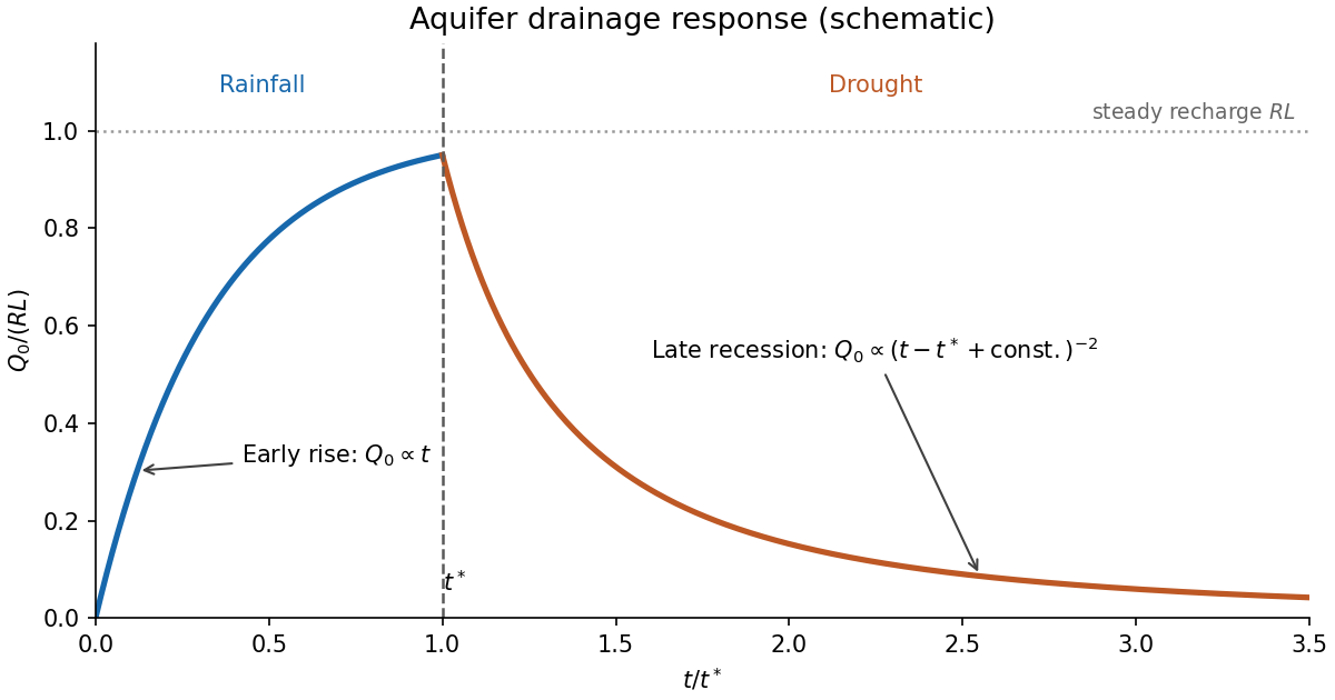
Let $J_X={\lim }_{x\downarrow 0}X(x)X^{\prime }(x)>0$. The spatial ordinary differential equation gives $(X{X}^{\prime }{)}^{\prime }=-\lambda X$, so its leading outlet behavior isAgain this is a square-root drainage boundary. For the separable aquifer drawdown, the dimensional drainage flux isEquivalently, with ${\tau }_d=\varphi /(K\lambda )$, it is $Q_0(t^{\ast })[1+(t-t^{\ast })/{\tau }_d{]}^{-2}$ for an exact separated profile. Integrating the spatial ordinary differential equation gives $J_X=\lambda {\int }_0^{L}Xdx$. This verifies the global mass conservation checkThus the late drainage flux follows an inverse-square power law, while stored water decays inversely with time.

The aquifer drainage hydrograph starts at zero, rises linearly in the early rainfall similarity solution, and approaches the total recharge $RL$ if rainfall lasts long enough for a finite-length steady state. Indeed, steady mass conservation gives $q_x=R$ and $q(L)=0$, hence $Q_0=RL$. At $t^{\ast }$, the outlet flux stays continuous for a regular inherited flux profile, then recedes as water drains; the eventual decay is proportional to $(t-t^{\ast }+\text{constant}{)}^{-2}$. An arbitrary transition requires the full time-dependent partial differential equation, so matching an early rainfall formula directly to a separated drought formula is only a schematic approximation.

The curve illustrates these regimes and a possible $t^{\ast }$. Its numerical shape and the relative duration of the regimes are schematic; the early rainfall and late drought formulas apply in their respective asymptotic ranges.