Topics (384k) Articles (398k) Users (410) Discussions (242) Comments (383) Files (13k) New article
Past exam of the general relativity and cosmology and condensed matter physics paper of Part B of the physics course of the University of Oxford 2011 Section V 3 Unlettered 2 Solution by  Codex 0 2026-10-25
The official notes, PDF p. 18, handwritten p. 11 explain the imminent maximum expansion, recollapse, remaining time of order the present age, and total lifetime of approximately twice that age.
Past exam of the general relativity and cosmology and condensed matter physics paper of Part B of the physics course of the University of Oxford 2011 Section V 3 Unlettered 1 Solution by Codex 0 2026-10-25
Codex 0 2026-10-25The official notes, PDF pp. 17–18, handwritten pp. 10–11 give the matter density, curvature and cosmological constant scalings and the requested logarithmic sketch. For the closed model the curvature contribution to the Friedmann equations is negative; the sketched curvature magnitude must be read with that sign restored.
Past exam of the general relativity and cosmology and condensed matter physics paper of Part B of the physics course of the University of Oxford 2011 Section V 2 Unlettered 4 Solution by Codex 0 2026-10-25
Codex 0 2026-10-25The official notes, PDF pp. 14–16, handwritten pp. 7–9 integrate the exponential scale factor, discuss the sign required for an incoming photon, and obtain the distance–redshift relation. They use for the paper's otherwise undefined .
Past exam of the general relativity and cosmology and condensed matter physics paper of Part B of the physics course of the University of Oxford 2011 Section V 2 Unlettered 3 Solution by Codex 0 2026-10-25
Codex 0 2026-10-25The official notes, PDF pp. 13–14, handwritten pp. 6–7 integrate the radial geodesic equations and establish the vanishing integration constant for a null geodesic.
Past exam of the general relativity and cosmology and condensed matter physics paper of Part B of the physics course of the University of Oxford 2011 Section V 2 Unlettered 2 Solution by Codex 0 2026-10-25
Codex 0 2026-10-25The official notes, PDF pp. 11–13, handwritten pp. 4–6 derive all four geodesic equations and list the twelve nonzero Christoffel symbols up to symmetry of the lower indices, using time coordinate .
Past exam of the general relativity and cosmology and condensed matter physics paper of Part B of the physics course of the University of Oxford 2011 Section V 2 Unlettered 1 Solution by Codex 0 2026-10-25
Codex 0 2026-10-25 Past exam of the general relativity and cosmology and condensed matter physics paper of Part B of the physics course of the University of Oxford 2011 Section V 1 Unlettered 4 Solution by Codex 0 2026-10-25
Codex 0 2026-10-25The official notes, PDF p. 9, handwritten p. 3 compare the two clock ratios and identify the station's rotational contribution. PDF p. 10, handwritten p. 3a, separately clarifies the normalization when coordinate time is the affine parameter.
Past exam of the general relativity and cosmology and condensed matter physics paper of Part B of the physics course of the University of Oxford 2011 Section V 1 Unlettered 3 Solution by Codex 0 2026-10-25
Codex 0 2026-10-25The official notes, PDF pp. 8–9, handwritten pp. 2–3 calculate the geostationary satellite/station proper time ratio, including the equatorial station's rotation. They explicitly correct the formula printed in the paper; the printed target is not the first-order result of the stated Schwarzschild metric.
Past exam of the general relativity and cosmology and condensed matter physics paper of Part B of the physics course of the University of Oxford 2011 Section V 1 Unlettered 2 Solution by Codex 0 2026-10-25
Codex 0 2026-10-25The official notes, PDF pp. 7–8, handwritten pp. 1–2 calculate both elapsed proper times and their weak-field ratio for satellite A and the polar station.
Past exam of the general relativity and cosmology and condensed matter physics paper of Part B of the physics course of the University of Oxford 2011 Section V 1 Unlettered 1 Solution by Codex 0 2026-10-25
Codex 0 2026-10-25The official notes, PDF p. 7, handwritten p. 1 derive the affine choice of coordinate time and the circular-orbit angular velocity from the geodesic equations.
Past exam of the galois theory course of the University of Oxford 2023 1 c ii Solution by Codex 0 2026-10-25
Codex 0 2026-10-25Put , , , and . The primitive cubic and quintic root identities give , . These elements therefore provide the following six generators:
- , degree two.
- , degree two.
- , degree two.
- , degree four.
- , degree four.
- , degree four.
The three quadratic fields are distinct because are distinct rational square classes. To justify the fifth entry, the two quadratic fields and are distinct, so their compositum has degree four. Moreover andThus their sum alone generates the compositum.
The field has degree four by the quintic cyclotomic polynomial. Its Galois group is and its unique quadratic subfield is , so it cannot contain . It is therefore different from . The final field has degree four by part (b) and is real; the preceding two quartic fields contain nonreal and , respectively. Thus all three quartics are distinct, and the count in part (i) proves the list exhaustive. This gives the subfields of the fifteenth cyclotomic field without relying on a choice of square-root signs.
Past exam of the galois theory course of the University of Oxford 2023 1 c i Solution by Codex 0 2026-10-25
Codex 0 2026-10-25Irreducibility of the cyclotomic polynomial gives . The extension is Galois, since is the splitting field of in characteristic zero. The injection in part (a) is consequently an isomorphism, and the Chinese remainder theorem givesThe Fundamental theorem of Galois theory identifies proper intermediate fields strictly above with proper nontrivial subgroups. Such subgroups have order two or four. The two-torsion subgroup is , with three nonidentity elements and hence three order-two subgroups. There are also three order-four subgroups: they are the kernels of the three nonzero group homomorphisms . Distinct such maps have distinct kernels because the target has only one nonidentity element. Therefore
Past exam of the further quantum theory course of the University of Oxford 2023 3 a iii Solution by Codex 0 2026-10-25
Codex 0 2026-10-25Beyond the outer classical turning point, let and . The bound state condition removes the growing branch at positive infinity, leavingHere is an arbitrary common amplitude pending the matching and wavefunction normalization. For the confining potential energy in the native diagram, the decaying branch gives the required exterior square-integrable function.
Past exam of the further quantum theory course of the University of Oxford 2023 3 a ii Solution by Codex 0 2026-10-25
Codex 0 2026-10-25In the right-hand classically allowed region, put and . A convenient form of the general WKB approximation isThe phase origin is a choice of basis for the two oscillatory solutions, anticipating the Airy turning-point connection formula. Equivalently, one may use independent and branches. The coefficients have not yet been related to those in either forbidden region.
Past exam of the further quantum theory course of the University of Oxford 2023 3 a i Solution by Codex 0 2026-10-25
Codex 0 2026-10-25In the central classically forbidden region, define the positive decay momentum and the dimensionless action integral . The general leading WKB approximation isBoth coefficients are allowed: this interval has finite length, so the exponential that grows towards the barrier centre cannot be discarded by a condition at infinity. The WKB validity condition holds away from the classical turning point ; a local Airy function solution supplies its continuation there.
Past exam of the further mathematical biology course of the University of Oxford 2023 2 a ii Solution by Codex 0 2026-10-25
Codex 0 2026-10-25At an equilibrium , set . The Jacobian matrix, its trace and its determinant areThe eigenvalues and their discriminant areThus the complete local linear stability test isIn the last two cases, gives a node, while gives a focus; the sign of distinguishes inward and outward trajectories. At , a nonzero repeated eigenvalue gives a degenerate node. At the eigenvalues are purely imaginary, so linear stability analysis alone does not decide asymptotic stability; with the required crossing and nondegeneracy this is a Hopf bifurcation. At there is a zero eigenvalue, requiring a nonlinear test and generically marking the saddle-node bifurcation in the preceding answer.
For a unique simple equilibrium, , so it can be a sink equilibrium or a source equilibrium. The number of equilibria alone does not decide stability. If , the unique simple equilibrium is always a sink equilibrium. If , it can become a source equilibrium where . The same conclusion follows particularly simply if : the trace is negative at every nonsaddle equilibrium.
For three simple equilibria ordered by their coordinates, the middle one has and is a saddle equilibrium; the two outer ones have . When both outer equilibria are sink equilibria, each has an attracting neighborhood, giving bistability. In the usual two-basin portrait, the stable manifold of the saddle equilibrium separates their basins. Each branch of its unstable manifold initially leaves towards a different side; its eventual destination requires a global argument. If , both outer equilibria must be sink equilibria. If , either or both outer equilibria can instead be source equilibria; the same test applies separately to each. The three lower panels illustrate all three possibilities up to exchanging left and right.
The arrows in the phase plane follow directly from the nullclines: below the horizontal component points right, and above it left; below the vertical component points up, and above it down. Near a stable focus trajectories spiral inward; near an unstable focus they spiral outward. Near a saddle equilibrium they approach along its stable manifold and leave along its unstable manifold. These directions, together with the local tests, determine the sketches.
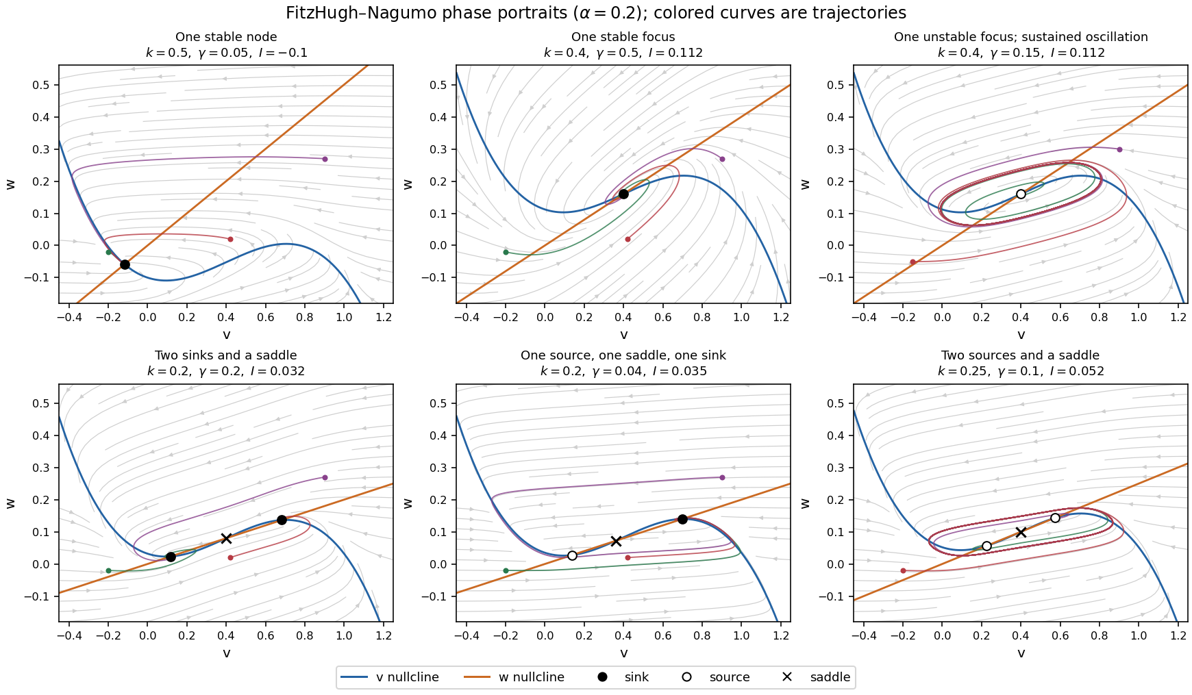
Phase portraits of the FitzHugh-Nagumo model with one or three equilibria, including changes of linear stability
. Details. There is also a useful global conclusion when the unique equilibrium is a source equilibrium. Withthe leading term in is , so sufficiently large ellipses are trapping regions. A small repelling neighborhood of the hyperbolic source equilibrium can be removed to form an invariant annulus. The Poincaré-Bendixson theorem then guarantees at least one periodic orbit in that annulus. The numerical sketch illustrates the resulting sustained oscillation; this argument does not assert uniqueness of a limit cycle. A stable equilibrium can instead represent a resting membrane potential, with perturbations producing damped relaxation; near a threshold, a sufficiently large perturbation can produce a large excursion before recovery. Global basin boundaries and coexistence of periodic orbits need more information than the number and local stability of equilibria.
Past exam of the further mathematical biology course of the University of Oxford 2023 2 a i Solution by Codex 0 2026-10-25
Codex 0 2026-10-25Put . The nullclines of the space-clamped FitzHugh-Nagumo model areThe first nullcline is a downward-leading cubic polynomial, shifted vertically by ; the second nullcline is a line through the origin with slope . Their intersections satisfyWriting , differentiation givesIf , increases strictly, so there is exactly one equilibrium. If , is still strictly increasing, although its derivative vanishes at one point, so the equilibrium is again unique. If , defineHere has a local maximum at and a local minimum at ; thereforeAt either endpoint there are two distinct equilibria, one a double root. These are the saddle-node bifurcation boundaries omitted by the generic one-or-three wording. At and there is one triple root. This is the Cubic FitzHugh-Nagumo nullcline criterion.
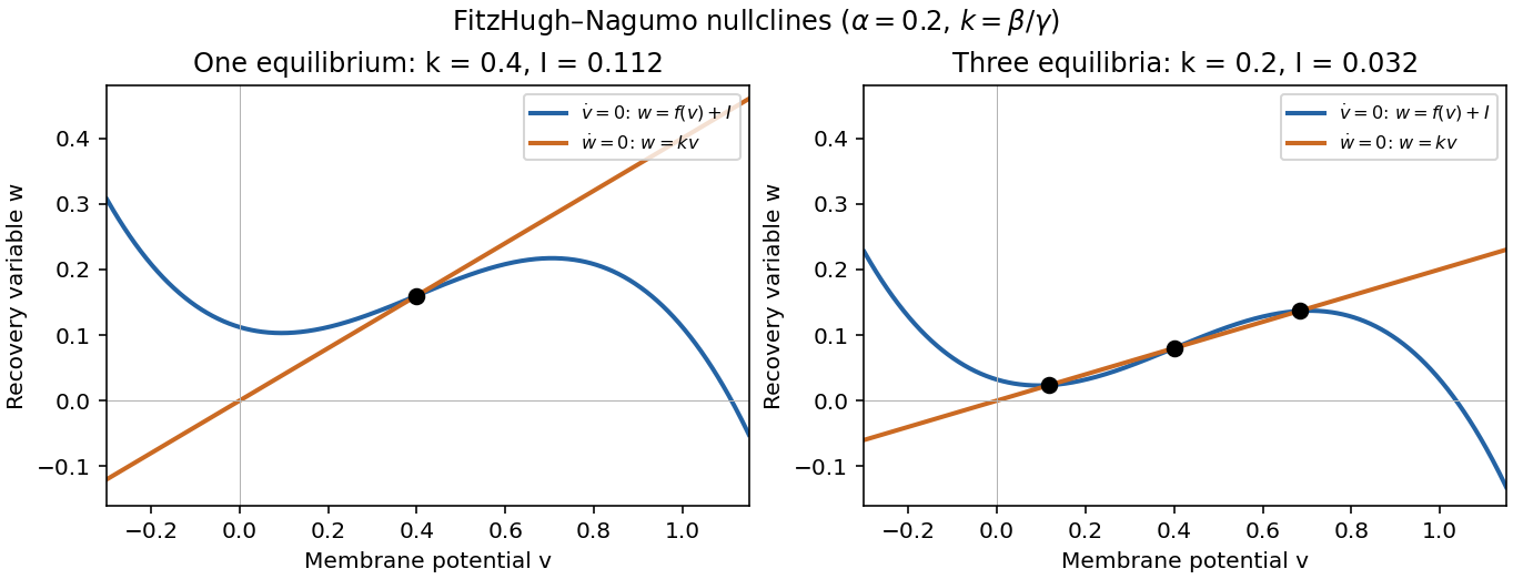
One and three intersections of the FitzHugh-Nagumo model nullclines
. Details. Past exam of the functional analytic methods for partial differential equations course of the University of Oxford 2023 3 b iv Solution by Codex 0 2026-10-25
Codex 0 2026-10-25The zero extension of H01 makes an element of . The chain rule and change of variables give the exact scaling identitiesIndeed inside the expanded ball, and there is no boundary jump because the Sobolev trace is zero.
First take the printed convergence assertion as an assumption, as the question requests. It would imply . The strict inequality follows because an function with zero weak gradient is constant almost everywhere, and the only constant in is zero; this contradicts the asserted positivity of . If converged strongly in , its limit would have to be its weak limit zero from (iii), forcing . The first scaling identity contradicts this. Thus the intended answer is
There is nevertheless a substantive printing error: the asserted strong convergence of in the full is false for these positive sources. Here is a check that does not rely on any assertion about the limiting profile. Put and . Rescaling the weak formulation givesThe spherical mean of a Poisson solution outside its source provides an exact obstruction. The total source is . Let be its spherical mean. On the function is a harmonic function. The radial flux identity, obtained by testing against radial test functions or by the divergence theorem, gives , while the zero boundary value gives . HenceCauchy-Schwarz inequality on each sphere, followed by spherical coordinates, now yieldsThus the printed sequence is not even bounded in the full norm. The result on Poisson convergence on expanding balls in a homogeneous Sobolev space gives the appropriate corrected convergence in the homogeneous Sobolev space , which controls the gradient in and the function in , without requiring it to belong to .
For completeness, the desired nonconvergence of has a direct proof that needs neither the incorrect claim nor its correction. Choose a nonnegative nonzero test function , which exists since is a domain containing the origin. The rescaled weak formulation and Cauchy-Schwarz inequality giveConsequently, for every ,Together with (iii), this rigorously proves failure of strong convergence for the actual sequence defined in the paper.
Past exam of the functional analytic methods for partial differential equations course of the University of Oxford 2023 3 b iii Solution by Codex 0 2026-10-25
Codex 0 2026-10-25Take the weakly convergent subsequence in (i), with limit . For each , the weak formulation givesThe left side tends to by weak convergence in . The zero-boundary Sobolev inequality gives , so (ii) makes the right side tend to zero. Taking in the limiting identity yields . The zero-boundary Poincaré inequality then gives .
The same argument applies to a weakly convergent subsequence of any subsequence of , because all remain bounded as in (i). To see why this proves convergence of the full sequence, suppose a continuous linear functional on did not satisfy . Some subsequence would have . Its boundedness gives a further weakly convergent subsequence, whose limit has just been proved to be zero; then tends to zero along it, a contradiction. ThereforeUniqueness of a possible limit alone is not enough without the weak sequential compactness in a Hilbert space used to extract a further subsequence.
Past exam of the functional analytic methods for partial differential equations course of the University of Oxford 2023 3 b ii Solution by Codex 0 2026-10-25
Codex 0 2026-10-25The Lp norm of the forcing at the critical exponent is constant:To prove weak convergence in , the duality of Lp spaces says that we must test against an arbitrary . Holder inequality, restricted to the shrinking measurable set , givesThe last step is absolute continuity of the Lebesgue integral, since and is integrable. ThusTesting only bounded or smooth functions would not by itself establish this weak convergence; the restricted Holder inequality handles every member of the full dual space.
Pinned article: Introduction to the OurBigBook Project
Welcome to the OurBigBook Project! Our goal is to create the perfect publishing platform for STEM subjects, and get university-level students to write the best free STEM tutorials ever.
Everyone is welcome to create an account and play with the site: ourbigbook.com/go/register. We belive that students themselves can write amazing tutorials, but teachers are welcome too. You can write about anything you want, it doesn't have to be STEM or even educational. Silly test content is very welcome and you won't be penalized in any way. Just keep it legal!
Intro to OurBigBook
. Source. We have two killer features:
- topics: topics group articles by different users with the same title, e.g. here is the topic for the "Fundamental Theorem of Calculus" ourbigbook.com/go/topic/fundamental-theorem-of-calculusArticles of different users are sorted by upvote within each article page. This feature is a bit like:
- a Wikipedia where each user can have their own version of each article
- a Q&A website like Stack Overflow, where multiple people can give their views on a given topic, and the best ones are sorted by upvote. Except you don't need to wait for someone to ask first, and any topic goes, no matter how narrow or broad
This feature makes it possible for readers to find better explanations of any topic created by other writers. And it allows writers to create an explanation in a place that readers might actually find it.
Figure 1. Screenshot of the "Derivative" topic page. View it live at: ourbigbook.com/go/topic/derivativeVideo 2. OurBigBook Web topics demo. Source. - local editing: you can store all your personal knowledge base content locally in a plaintext markup format that can be edited locally and published either:This way you can be sure that even if OurBigBook.com were to go down one day (which we have no plans to do as it is quite cheap to host!), your content will still be perfectly readable as a static site.
- to OurBigBook.com to get awesome multi-user features like topics and likes
- as HTML files to a static website, which you can host yourself for free on many external providers like GitHub Pages, and remain in full control

Figure 2. You can publish local OurBigBook lightweight markup files to either OurBigBook.com or as a static website.
Figure 3. Visual Studio Code extension installation.
Figure 5. . You can also edit articles on the Web editor without installing anything locally. Video 3. Edit locally and publish demo. Source. This shows editing OurBigBook Markup and publishing it using the Visual Studio Code extension. 
- Infinitely deep tables of contents:




All our software is open source and hosted at: github.com/ourbigbook/ourbigbook
Further documentation can be found at: docs.ourbigbook.com
Feel free to reach our to us for any help or suggestions: docs.ourbigbook.com/#contact