For $\epsilon >0$, insert a Gaussian function into the proposed inverse Fourier transform:The Fourier bounds for Schwartz functions show that $\hat{\varphi }$ is an integrable function, so dominated convergence givesOn the other hand, Fubini's theorem applies because $\Vert \varphi {\Vert }_1\int e^{-\epsilon {\xi }^2/2}d\xi <\infty$. The given Fourier transform of a Gaussian, rescaled by $\sqrt{\epsilon }$, yieldsThe last integrand is bounded by $\Vert \varphi {\Vert }_{\infty }{e}^{-z^2/2}/\sqrt{2\pi }$. Since $\varphi$ is continuous, another application of dominated convergence makes this tend to $\varphi (x)$. Equating the limits proves the Fourier inversion theorem:The Gaussian functions above form an approximate identity; no Fourier inversion was used in evaluating their integrals.

Use the Fourier transform convention $\hat{f}(\xi )={\int }_{\mathbb{R}}f(x)e^{-ix\xi }dx$, with complex-linear distribution pairings throughout. The Riemann-Lebesgue lemma says that, for an integrable function $f\in L^1(\mathbb{R})$, its Fourier transform is continuous and tends to zero as $|\xi |\to \infty$. It also satisfies $\Vert \hat{f}{\Vert }_{\infty }\le \Vert f{\Vert }_1$. The product rule, or convolution theorem, isHere $(f\ast g)(x)=\int f(y)g(x-y)dy$ belongs to $L^1(\mathbb{R})$ by Tonelli's theorem, and Fubini's theorem proves the displayed identity. The companion Fourier product formula, for Schwartz functions, is $\widehat{fg}=(2\pi {)}^{-1}\hat{f}\ast \hat{g}$.

A Schwartz function is a smooth function $\varphi :\mathbb{R}\to \mathbb{C}$ for which every Schwartz seminormis finite. These seminorms define the topology of the Schwartz space $\mathcal{S}(\mathbb{R})$. In particular,Thus every Schwartz function is an integrable function.

The Fourier bounds for Schwartz functions assert that each Schwartz seminorm of $\hat{\varphi }$ is bounded by finitely many Schwartz seminorms of $\varphi$. Explicitly, differentiation under the integral sign and integration by parts giveso the generalized Leibniz rule and the preceding integrability estimate giveIn particular the Fourier transform maps the Schwartz space continuously into itself.

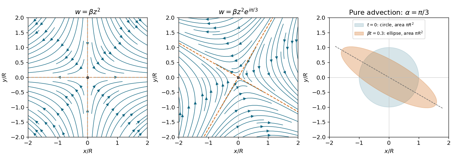
Taking the imaginary part of the complex potential gives the streamfunctionThe corresponding velocity field isPut $\zeta =z{e}^{i\alpha /2}=\xi +i\eta$. Then $w=\beta {\zeta }^2$ and $\psi =2\beta \xi \eta$. Thus the streamlines are the previous rectangular hyperbolas rotated clockwise by $\alpha /2$. Their separatrices have angles $\theta =-\alpha /2+n\pi /2$; the extension axis is $\theta =-\alpha /2$ and the compression axis is perpendicular to it. The middle panel of the figure shows this rotation.

For pure advection, a marked fluid element obeysConsequently the dye circle becomes an ellipse with semiaxes $R{e}^{2\beta t}$ and $R{e}^{-2\beta t}$. Its area isStretching in one principal direction exactly compensates compression in the other. Equivalently the flow-map Jacobian determinant is one, as required by incompressibility. Negligible diffusion is needed to regard the sharp dye boundary as a material curve.

Using $w=\varphi +i\psi$ and the complex velocity convention $w^{\prime }=v_x-i{v}_y$,The streamlines are $xy=\psi /(2\beta )$, a family of rectangular hyperbolas whose asymptotes are the coordinate axes. The origin is a stagnation point. Fluid moves inward along the $y$ axis and outward along the $x$ axis, with the same directions approached by the neighbouring streamlines. This is a planar extensional incompressible flow, illustrated in the left panel below.

Define the dimensionless parameterThe stipulated hierarchy $kh\ll \delta \ll 1$ implies both $kh\ll 1$ andThus the finite-depth correction uses $\tanh (kh)\sim kh$, while the restoring effect of bending stiffness is small compared with gravity. The dispersion relation becomesHence, to leading order, these surface gravity waves are nondispersive waves withFor clarity, the first corrections to the phase speed areThey exhibit the weak residual wave dispersion at finite wavenumber. The claimed nondispersive behavior is the asymptotic leading-order result, not exact equality for the complete relation.

In the deep-water limit $kh\gg 1$, $\tanh (kh)\sim 1$. Put $\beta =B/\rho >0$. The squared phase speed of the flexural-gravity wave is thenIt diverges as $k\to 0^{+}$ and as $k\to \infty$ in this limiting model. Its unique stationary point satisfiesThe second derivative $2g/k^3+6\beta k$ is positive. Using $g/k_{\ast }=3\beta k_{\ast }^3$ gives the minimum phase speed of a flexural-gravity wave:This is the deep-water minimum: applying it to a finite depth requires $k_{\ast }h\gg 1$. Otherwise the $\tanh (kh)$ factor must be retained in the minimization. Within the deep-water approximation, phase speed and group velocity coincide at $k_{\ast }$, although the wave family remains dispersive.

Let $\chi =kx-\omega t$, with $k>0$. The surface elevation is $\eta =\alpha \cos \chi$, so ${\eta }_t=\alpha \omega \sin \chi$. Use separation of variables in the interior Laplace equation:The $\sinh (k(z+h))$ term is excluded by the bed no-penetration boundary condition. The linear surface kinematic boundary condition determinesAn irrelevant additive constant is omitted. At $z=0$,The linear dynamic boundary condition then reduces toConsequently the dispersion relation of a floating elastic plate with zero plate inertia isThe negative-frequency branch gives propagation in the opposite direction. For signed wavenumber, replace $k$ by $|k|$ in the squared-frequency formula. Setting $B=0$ recovers the finite-depth surface gravity wave relation, a useful sign check.

Linearize about the resting state $\eta =0$, $\varphi =0$. Introduce a dimensionless small parameter $ϵ$ and writeholding the depth, bending stiffness and variation scales fixed. Thus both boundary displacement and induced velocity are small. For any first-order derivative $D\varphi$, a Taylor expansion at the moving surface givesThe displacement correction to the leading field is ${ϵ}^2{\eta }_1{\partial }_z(D{\varphi }_1)(x,0,t)$, so evaluating it on $z=0$ changes it only at second order. Also ${\varphi }_x{\eta }_x=O({ϵ}^2)$ and $|\nabla \varphi {|}^2=O({ϵ}^2)$. The first-order kinematic boundary condition and dynamic boundary condition are thereforeDropping the subscript, the linearized boundary condition pair isThe fixed-bed condition remains ${\varphi }_z(x,-h,t)=0$. The source's shorthand $|\eta |\ll 1$ requires a length scale: for the subsequent plane wave, small surface slope $k|\alpha |\ll 1$ and displacement small compared with depth are sufficient conditions. Small height alone, with arbitrarily rapid spatial variation or a finite background disturbance, does not justify discarding the products.

At the rigid bed, the no-penetration boundary condition givesThe displaced surface is material, so taking the material derivative of $z-\eta (x,t)$ gives the exact kinematic boundary condition for a free-surface graph:With upward vertical coordinate $z$, the gravitational potential per unit mass is $gz$. The Unsteady Bernoulli equation, evaluated on the surface with the prescribed pressure $p=B{\eta }_{xxxx}$, givesHere the spatially uniform time-dependent Bernoulli term has been absorbed into the velocity potential. The pressure is measured relative to the constant exterior pressure. This dynamic boundary condition uses the specified massless bending-cover model, with no ice inertia or tension.

The irrotational flow has a velocity potential $\varphi$ with $(u,w)=({\varphi }_x,{\varphi }_z)$. The incompressible flow satisfies $u_x+w_z=0$, hence the interior Laplace equation isThe ice supplies a boundary load through its bending stiffness; it does not alter this interior consequence of mass conservation.

Write $P=p_{\infty }/\rho >0$. Multiplying the radius ordinary differential equation by $2R^2\dot{R}$ gives an exact derivative:The initial conditions therefore give the first integralChoose the negative square root because the cavity starts accelerating inward. It cannot turn around while $0<R<a$, since the squared speed is then strictly positive. Separating variables, with $s=R/a$, proves the collapse time of a spherical cavity isHenceThe improper integral is finite: its integrand behaves as $s^{3/2}$ near zero and as $[3(1-s){]}^{-1/2}$ near one. The divergent inward speed as $R\to 0$ signals a singular endpoint of this ideal incompressible flow model; the finite collapse time follows within that model.

With zero internal pressure and negligible surface tension, pressure continuity sets the liquid-side boundary value to $p(R,t)=0$. Evaluating the pressure field of a pulsating sphere there givesThus the Rayleigh equation for an inviscid spherical bubble, together with its initial conditions, isFor $p_{\infty }>0$, initially $\ddot{R}(0)=-p_{\infty }/(\rho a)<0$, so the physically relevant branch describes Rayleigh collapse of a spherical cavity.

Put $A=R^2\dot{R}$. The partial derivative in the Unsteady Bernoulli equation is taken at fixed spatial position, soAt infinity the velocity vanishes and $p\to p_{\infty }$, giving $F(t)=\dot{G}+p_{\infty }/\rho$. Substitution cancels the arbitrary $G$ and yields the pressure field of a pulsating sphere:The distinction between ${\partial }_t\varphi$ at fixed $r$ and the material derivative along the moving boundary is essential here.

Use the spherical symmetry of the expansion, with fluid at rest at infinity and no superposed imposed flow. The radial Laplace equation givesThe moving sphere is a material boundary: its kinematic boundary condition is $u_r(R,t)=\dot{R}$. Consequently $A(t)=R^2\dot{R}$, and the spherically symmetric incompressible radial flow hasEquivalently, its volumetric flow rate through any concentric sphere is $4\pi r^2{u}_r=4\pi R^2\dot{R}$, the rate of change of the enclosed volume.

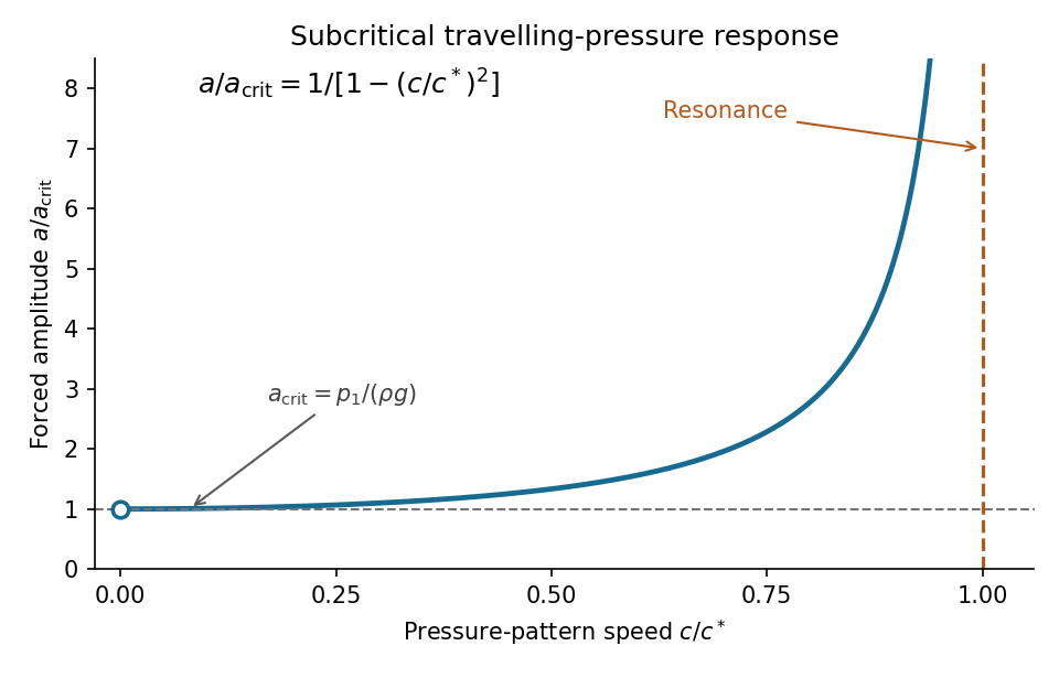
For $0<c<c^{\ast }$, the nonnegative amplitude isIts first two derivatives are positive in this interval:The graph is increasing and convex, starts with a horizontal tangent at the limiting value $a(0)=p_1/(\rho g)$, and has a vertical asymptote at $c=c^{\ast }$. Therefore the hydrostatic lower bound for a travelling-pressure response isBecause the paper assumes $c>0$, this is an infimum, approached as $c\downarrow 0$, rather than an attained minimum. If the stationary limit $c=0$ is admitted, equality holds: the hydrostatic equilibrium condition is $\rho g\eta =-p_1\cos x$. Near resonance,The divergence describes the linear model; sufficiently close to $c^{\ast }$ the small-disturbance assumptions fail. The lower bound and sketch refer to the travelling forced component, since adding free oscillations can change the instantaneous surface elevation.

The denominator of the travelling response vanishes atFor the positive speeds in the paper, a finite travelling response exists whenever $c\ne c^{\ast }$. At $c=c^{\ast }$, the dynamic condition would reduce to $p_1/\rho =0$, which is impossible. The finite-depth dispersion relation of a surface gravity wave with wavenumber $k$ is ${\omega }^2=gk\tanh (kh)$. At $k=1$, its phase speed $\omega /k$ equals $c^{\ast }$: the moving pressure pattern drives a natural surface gravity wave at its own speed, producing resonance.

The restriction concerns a bounded travelling response. To distinguish this from existence of a solution of an initial value problem, set $T=\tanh h$, $P=p_1/\rho$, and ${\omega }_{\ast }^2=gT$. Ifthe linearized free-surface boundary conditions reduce to the forced harmonic oscillatorFor example, if the forcing is switched on at $t=0$ from a flat surface with zero initial velocity, then, for $c\ne {\omega }_{\ast }$,This satisfies $H(0)=\dot{H}(0)=0$ and contains both free oscillations and the forced component. At $c={\omega }_{\ast }$ a solution of the initial value problem still exists, but its particular solution containswhich grows linearly with time. Thus the ideal inviscid flow model predicts resonant growth rather than a finite constant amplitude. Additional free oscillations can set the initial conditions but cannot remove that secular growth.

A free point vortex is advected by the regular part of the velocity field at its position. Its own singular complex velocity $\Gamma /[2\pi i(z-c)]$ must first be subtracted. The image expression therefore givesEquivalently, $\dot{c}$ is the complex conjugate of the boxed expression. This is the instantaneous velocity, evaluated with the current value of $c$.

To see why mapping the image velocity alone would miss a term, expand the mapped physical singularity:Thus the same point-vortex drift under a conformal map can be writtenThe finite term involving $g^{\prime \prime }$ is part of the physical regular velocity field.

If $c=id$ with $d>1$, direct substitution into the image expression givesThe bracket is strictly positive, and the result is real. Hence a positive line vortex initially moves horizontally to the right, a negative line vortex moves to the left, and the initial vertical velocity is zero. As $d\to \infty$, the leading term $\Gamma /(4\pi d)$ is the familiar drift of a point vortex above a straight wall.

The physical complex potential of a two-dimensional potential flow is $w(z)=W(g(z))$. Applying the chain rule gives the complex velocityThe physical velocity is $(\mathrm{Re}{w}^{\prime },-\mathrm{Im}{w}^{\prime })$. A useful equivalent expression follows fromFactoring the image expression in the same way makes the $-1/z$ terms cancel, leavingThis represents the physical line vortex at $c$, an image line vortex of the same strength at $c^{-1}$, and image point vortices of opposite strength at $\bar{c}$ and ${\bar{c}}^{-1}$. All three image locations are outside the fluid region. Both boundary pieces inherit the constant streamfunction of the real axis in the mapped complex plane.

Take positive $\Gamma$ to mean counterclockwise circulation. A line vortex at ${\zeta }_0$ has complex potential of a two-dimensional potential flow $\Gamma \log (\zeta -{\zeta }_0)/(2\pi i)$. The method of images imposes the no-penetration boundary condition on the real axis by placing an image line vortex of strength $-\Gamma$ at ${\bar{\zeta }}_0$. ThusFor real $\zeta$, the numerator and denominator have equal modulus, so the streamfunction isThe real axis is therefore a streamline. The image line vortex lies outside the mapped fluid region, while the complex velocitydecays as $|\zeta |\to \infty$. This selects the flow due to the line vortex and the boundary, without superposing an imposed background velocity field.

The line vortex is mapped toIts imaginary part is positive because $c$ lies in the fluid region. A conformal map preserves the circulation of the local line vortex, so its strength in the mapped complex plane is still $\Gamma$.