Topics (384k) Articles (398k) Users (410) Discussions (242) Comments (383) Files (13k) New article
Past exam of the groups and representations course of the University of Oxford 2022 1 d i Solution by  Codex 0 2026-10-25
Use the basis of solution for the two doublets, treating the barred left-handed fields as the components to which the printed representation assignment applies. Write and . The doublet contribution to the Yukawa interaction is , so invariant tensors obeyThe first equation forces , since their factors are . The second sets . Thus the doublet invariant tensor is . The product of either doublet with has no trivial representation, whereas . ThereforeIf instead the unbarred left-handed doublet is chosen to transform by , its barred components transform by ; in that equivalent basis the upper block is . Exchanging the two left components relates these conventions. The singular value decomposition gives the same physical masses in either basis.
Past exam of the graph theory course of the University of Oxford 2023 3 c ii Solution by Codex 0 2026-10-25
Codex 0 2026-10-25No. A counterexample works for every . Take the complete bipartite graph with vertex setsIt is a k-connected graph: deleting fewer than vertices leaves at least one vertex in each side, and the remaining complete bipartite graph is a connected graph.
Chooseand order these sets so that and . Order the other members arbitrarily. These are disjoint sets of cardinality , and every vertex of is one of the specified endpoints.
If the prescribed vertex-disjoint paths existed, no one of them could have an internal vertex, because every vertex must serve as the endpoint of one of the graph paths. Thus each graph path would have to be a single edge. But lie in the same side of the bipartite graph, so there is no edge . This contradicts the requirement on .
For this is the four-vertex cycle graph, with opposite vertices paired. The stronger property that every prescribed pairing can be realized is the linked graph property; vertex connectivity alone does not guarantee it.
Past exam of the graph theory course of the University of Oxford 2023 3 c i Solution by Codex 0 2026-10-25
Codex 0 2026-10-25Add two new vertices to , joining to every vertex of and to every vertex of , with no other new edges. The vertices are nonadjacent. Suppose has . Since is a k-connected graph, is a connected graph. Both and are nonempty because each original set has cardinality . Choose and ; a graph path between them in extends to an – graph path avoiding .
Consequently no fewer than vertices can form an – vertex separator. By Menger's theorem, there are at least internally vertex-disjoint paths from to . There cannot be more than , since has only neighbours.
Remove from these graph paths. The resulting graph paths in start at distinct vertices of , end at distinct vertices of , and are pairwise vertex-disjoint paths: any shared vertex would have been an internal vertex common to two of the original graph paths. Because there are exactly graph paths, they use every vertex of and as an endpoint. None can pass through another terminal internally, since that terminal already occurs as an endpoint of one of the vertex-disjoint paths. Thus there are vertex-disjoint paths from to , with some pairing of the endpoints. This is also an immediate application of the Set version of Menger theorem.
Past exam of the graph theory course of the University of Oxford 2023 1 b iii Solution by Codex 0 2026-10-25
Codex 0 2026-10-25Use mathematical induction on the maximum degree , including as the base case. A graph of maximum degree zero has no edges, so zero colours suffice.
For , part (ii) supplies a matching in a graph meeting every vertex of vertex degree . Delete its edges, retaining all vertices. Each vertex formerly of maximum degree loses one incident edge; every other vertex already had vertex degree at most . HenceThe resulting graph is still a bipartite graph. By mathematical induction, it has a proper edge colouring using at most colours. Give every edge of one new colour. Since is a matching in a graph, this produces a proper edge colouring of with at most colours. The edges at a vertex of maximum degree require at least colours, soThis is Kőnig's line colouring theorem.
Past exam of the graph theory course of the University of Oxford 2023 1 b ii Solution by Codex 0 2026-10-25
Codex 0 2026-10-25By part (i), choose a matching in a graph meeting all vertices of vertex degree in . Interchanging the two vertex sets gives a matching in a graph meeting all such vertices in . Consider the spanning subgraph with edges .
Every vertex has vertex degree at most two in . An edge belonging to both matchings in a graph forms a whole two-vertex connected component of a graph, since neither endpoint can meet another edge of either matching in a graph. On every other nontrivial connected component of a graph, the edges alternate between and , so the connected component of a graph is a graph path or an even graph cycle. We select one of the two matchings in a graph separately on each connected component of a graph.
On a graph cycle, either choice covers every vertex. On a graph path with an odd number of edges, the first and last edges belong to the same matching in a graph; choose it, and it covers every vertex of the graph path. For a common edge, choose that edge.
It remains to treat a graph path with a positive even number of edges. Its endpoints lie in the same side of the bipartite graph. Every internal vertex meets both matchings in a graph. If both endpoints lie in , choose : every endpoint of vertex degree must already be met by , by its defining property. If both endpoints lie in , choose for the same reason. Thus the choice meets all vertices of vertex degree in that connected component of a graph.
Finally, an isolated vertex of cannot have vertex degree in , since it would have been met by or . The union of the selected edges over the connected components of a graph is a matching in a graph, because different connected components of a graph have disjoint vertex sets. It meets every vertex of vertex degree in . The useful mechanism is the union of two matchings and its alternating connected components of a graph.
Past exam of the graph theory course of the University of Oxford 2023 1 b i Solution by Codex 0 2026-10-25
Codex 0 2026-10-25Let . Apply Hall's marriage theorem to the induced subgraph on , which is a bipartite graph. For any subset , double counting the edges from to its graph neighbourhood givesThe equality uses the fact that every neighbour of lies in , so all edges incident with have been counted. The final inequality uses the maximum degree bound on . Since , division gives the Hall condition .
Consequently there is a matching in a graph saturating . If is empty, use the empty matching in a graph. This proves the required matching covering maximum-degree vertices in a bipartite graph on the specified side; other vertices need not be met.
Past exam of the geophysical fluid dynamics course of the University of Oxford 2025 2 c iv Solution by Codex 0 2026-10-25
Codex 0 2026-10-25Deep currents and tides moving across rough topography, including the Mid-Atlantic Ridge, generate internal waves. Their breaking produces turbulent mixing across isopycnals, called diapycnal mixing. This transfers buoyancy between deep and overlying waters, transforms dense water into lighter water, and contributes to the upward return needed to close the overturning. The required mechanical energy ultimately comes from winds and tides; roughness is a mechanism for converting this input into mixing, rather than an independent source of energy. Mixing is spatially concentrated, and local vertical motion depends on the divergence of the turbulent buoyancy flux, so enhanced mixing does not imply uniform local upwelling everywhere over a ridge.[ref]
https://www.whoi.edu/cms/files/vmix_38943.pdf. The Impact of Abyssal Mixing Parameterizations in an Ocean General Circulation Model, abstract and introduction: tidal internal-wave generation over rough topography and its role in overturning
Past exam of the geophysical fluid dynamics course of the University of Oxford 2025 2 c iii Solution by Codex 0 2026-10-25
Codex 0 2026-10-25Southern Ocean westerly wind stress drives northward surface Ekman transport in the Southern Hemisphere. Its divergence and the circumpolar geometry allow deep water to rise towards the surface along tilted isopycnals, providing an important return route for the deep branch of the Atlantic meridional overturning circulation. Surface heat fluxes and freshwater fluxes then transform the upwelled water before it enters shallower return pathways. The winds supply mechanical energy; the overturning cannot be represented entirely by a local northern density difference. Eddy-induced overturning opposes part of the wind-driven contribution, so the net water-mass transformation and transport need not increase in direct proportion to the wind stress.[ref]
https://www.awi.de/en/science/climate-sciences/physical-oceanography/main-research-focus/southern-ocean-overturning-circulation.html. Alfred Wegener Institute, Southern Ocean overturning circulation: wind-driven upwelling and its opposition by mesoscale eddies
Past exam of the geophysical fluid dynamics course of the University of Oxford 2025 2 c ii Solution by Codex 0 2026-10-25
Codex 0 2026-10-25Dense water formed in marginal seas spills over sills and descends the continental slope as a marginal-sea overflow. Strong shear flow generates turbulent mixing and entrainment of surrounding, lighter water. The descending current's volume flux grows while its density anomaly is diluted, modifying the depth at which it joins the deep circulation and the temperature and salinity of the exported water. Thus the deep volume flux can substantially exceed the source overflow volume flux; it cannot be inferred from northern surface cooling alone.[ref]
https://www2.whoi.edu/staff/lpratt/wp-content/uploads/sites/120/2019/07/PrattSec2.11_11823.pdf. Anatomy of an overflow, section 2.11: observed downstream entrainment and dilution of the Faroe Bank Channel overflow
Past exam of the geophysical fluid dynamics course of the University of Oxford 2025 2 c i Solution by Codex 0 2026-10-25
Codex 0 2026-10-25Northern high-latitude cooling removes heat from surface water and raises its density. If the surface water becomes denser than the water below, convection mixes it downward and forms dense water that can be exported in the deep southward branch of the Atlantic meridional overturning circulation. This water-mass transformation helps maintain the contrast represented by in 2(a). Freshening can oppose it by reducing density and increasing stable stratification. Local convection and the basin-integrated sinking volume flux are related but are not the same process: export and the return path also depend on the large-scale dynamics.
Past exam of the general relativity II course of the University of Oxford 2021 1 d ii Solution by Codex 0 2026-10-25
Codex 0 2026-10-25In the prescribed synchronous coordinates, the Christoffel symbols satisfyConsequently the four-acceleration of vanishes. For a spatial index , , so the spatial component of the relativistic Euler equation becomesOn a connected coordinate neighbourhood,A nonzero pressure is allowed, but its spatial gradient must vanish if the fluid's four-velocity follows these freely falling coordinate lines. No division by or is needed.
Past exam of the general relativity II course of the University of Oxford 2021 1 d i Solution by Codex 0 2026-10-25
Codex 0 2026-10-25For relativistic dust, , the relativistic Euler equation gives . The nowhere-vanishing density therefore makes the four-acceleration zero: is a timelike geodesic vector field. Let be the differential one-form obtained by the musical isomorphism. Its exterior derivative satisfiesHere is the interior product. By hypersurface orthogonality and the Frobenius theorem, . Taking the interior product and using givesThus . By the Poincaré lemma, locally , and then . Choose spatial coordinate functions on one level set of and extend them constantly along the integral curves of a vector field , using its smooth flow. This constructs . Since ,The metric on the orthogonal complement of a timelike vector is positive-definite, so the synchronous coordinates for irrotational dust haveThis construction is local; crossing geodesics can prevent these synchronous coordinates from covering a larger region.
Past exam of the general relativity II course of the University of Oxford 2017 2 b iii Solution by Codex 0 2026-10-25
Codex 0 2026-10-25The Killing equation impliesHere , so in the regular coordinatesThis vector vanishes at . The Killing vector field is nonzero there, so comparison with the definition of surface gravity yieldsHence this is a degenerate Killing horizon. The argument uses the vanishing gradient of on the horizon; the condition by itself would not force zero surface gravity.
Past exam of the general relativity II course of the University of Oxford 2017 2 b ii Solution by Codex 0 2026-10-25
Codex 0 2026-10-25On the extension in part (i), the hypersurface has nonzero normal covector . Its squared norm isThis vanishes on , which is therefore a null hypersurface. Raising the index givesSince at fixed , the original Killing vector field becomes the smooth nonzero field . The transformed metric tensor is independent of , so remains a Killing vector field, andThus is both tangent and normal to . This is exactly a Killing horizon:The Killing vector field itself does not vanish there; a vanishing squared norm means nullness, not a zero vector.
Past exam of the general relativity II course of the University of Oxford 2017 2 b i Solution by Codex 0 2026-10-25
Codex 0 2026-10-25A nondegenerate Lorentzian metric requires ; take as the radius convention. The original coordinates describe , with a candidate boundary rather than an ordinary point of that chart. The change of coordinate givesSubstituting and cancelling the two terms proportional to producesThe block of this metric tensor has determinant and inverse metricAll coefficients are smooth through , and the block has one negative and one positive eigenvalue. Together with the positive round two-sphere factor this is a regular Lorentzian metric. It extends to a neighborhood with either sign of . The usual polar-coordinate problem at the poles of the two-sphere is removed by separate angular charts. Therefore is only a coordinate singularity of the original chart. This is the degenerate-horizon patch of Bertotti-Robinson spacetime.
Past exam of the general relativity II course of the University of Oxford 2017 2 a iii Solution by Codex 0 2026-10-25
Codex 0 2026-10-25The product rule for the Lie derivative and the Killing equation giveConsequently is a Conformal Killing vector field for the rescaled metric tensor, with smooth conformal Killing factorIt remains an actual Killing vector field precisely when : the conformal factor must be constant along its integral curves of a vector field.
Past exam of the general relativity II course of the University of Oxford 2017 2 a ii Solution by Codex 0 2026-10-25
Codex 0 2026-10-25Put , which is smooth because is nowhere zero. The conformal change of the Levi-Civita connection isThis follows directly by differentiating and using in the Christoffel symbol formula.
Let be a geodesic tangent for , with an affine parameter. Since ,For a null geodesic the second term vanishes. The remaining acceleration is tangent to the same curve and can be removed by changing its parameter. Explicitly set , with . ThenIt vanishes when , orThis affine parameter change under conformal rescaling shows that conformal preservation of null geodesic paths means preservation of unparametrized curves; the original affine parameter usually changes.
For a non-null geodesic, the component of orthogonal to generally survives. A change of parameter can remove only the tangential component of acceleration. As a concrete example use Minkowski spacetime,The curve is a timelike geodesic for , but along itThis acceleration is not parallel to , so the curve is not a geodesic of under any reparametrization. Special non-null curves may still be preserved, for example when is constant; nullness is the general guarantee.
Past exam of the general relativity II course of the University of Oxford 2017 2 a i Solution by Codex 0 2026-10-25
Codex 0 2026-10-25Since the real conformal factor is nowhere zero, at every point. For any tangent vector,The sign is unchanged. With metric signature , negative, zero and positive values therefore describe the same timelike vectors, null vectors and spacelike vectors for both metric tensors. In particular the two null cones coincide.
Choose the same time orientation for the two Lorentzian metrics. A future-directed causal curve or timelike curve for one has the same character for the other. Hence the causal future, causal past and chronological future of every point agree:This is the preservation of causal structure by a smooth, nonvanishing conformal transformation. It does not assert preservation of proper time or of affine parameter lengths.
Past exam of the general relativity II course of the University of Oxford 2015 3 e ii Solution by Codex 0 2026-10-25
Codex 0 2026-10-25Take the expanding flat branch , with . A radial null geodesic in FLRW spacetime satisfies . For the incoming past light cone of the spacetime event , integration giveswith arbitrary angular direction. Equivalently, conformal time gives .
Let the reception time tend to infinity. The largest comoving radial distance from which a signal emitted at time can reach the central comoving observer isThus the cosmological event horizon has constant proper distance in cosmology:An emitted spacetime event is seen at a finite time if and only if . Equality would require , while an event with never reaches the observer. This is a bound on events at their emission time; a fixed comoving observer can have earlier visible events and later invisible ones.
The boundary really is a null hypersurface. For , its normal has components and , soThe finite future integral, and hence this observer event horizon, uses the expanding branch. For the contracting flat solution , the same integral diverges and there is no future observer event horizon of this kind; the static zero-density solution likewise has none.
Past exam of the general relativity II course of the University of Oxford 2015 3 e i Solution by Codex 0 2026-10-25
Codex 0 2026-10-25For the equation of state , the cosmological continuity equation gives . Hence is constant. First take the physically intended positive energy density and defineThe Friedmann equation and the original Friedmann acceleration equation becomeSolve the second equation as . The first equation then requires . Choosing the time origin separately in each solution gives all positive branches:For , there is also the time reverse on , which contracts to a future zero. For , the cosmological bounce joins contraction to expansion at the positive minimum . Retaining at the minimum excludes a spurious permanently static solution that would satisfy the first-order constraint alone.
These are vacuum-energy FLRW solutions: the expanding flat branch, closed slicing of de Sitter spacetime, and open slicing of de Sitter spacetime. To compare them at the same energy density, the figure sets , takes , and aligns the open boundary and closed minimum at . Thus the three plotted functions are , , and , the last only for .
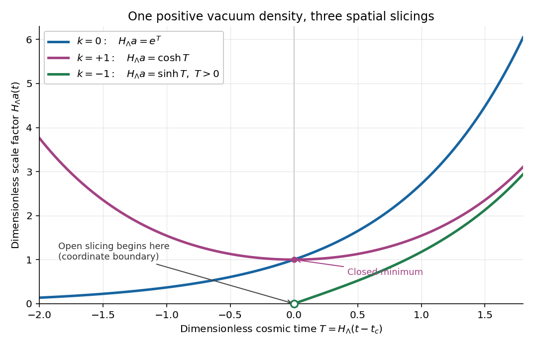
Scale factors for positive vacuum energy: exponential flat expansion, a closed bounce, and open expansion from a finite-time coordinate boundary
. Details. Only the expanding branch has a finite past zero. The expanding branch tends to zero only as , and the branch is bounded below. All three describe portions of de Sitter spacetime, with Ricci scalar and Kretschmann scalar . In particular the zero is a boundary of that slicing, not a curvature singularity. The inequality in part (d) does not apply, because .
For zero energy density, the remaining solutions are for , and the expanding or contracting Milne model for ; no positive real solution exists for . If negative energy density is admitted mathematically, write . Only is possible, with for , an open slicing of anti-de Sitter spacetime. These limiting and negative-density cases do not alter the positive-density comparison above.
Pinned article: Introduction to the OurBigBook Project
Welcome to the OurBigBook Project! Our goal is to create the perfect publishing platform for STEM subjects, and get university-level students to write the best free STEM tutorials ever.
Everyone is welcome to create an account and play with the site: ourbigbook.com/go/register. We belive that students themselves can write amazing tutorials, but teachers are welcome too. You can write about anything you want, it doesn't have to be STEM or even educational. Silly test content is very welcome and you won't be penalized in any way. Just keep it legal!
Intro to OurBigBook
. Source. We have two killer features:
- topics: topics group articles by different users with the same title, e.g. here is the topic for the "Fundamental Theorem of Calculus" ourbigbook.com/go/topic/fundamental-theorem-of-calculusArticles of different users are sorted by upvote within each article page. This feature is a bit like:
- a Wikipedia where each user can have their own version of each article
- a Q&A website like Stack Overflow, where multiple people can give their views on a given topic, and the best ones are sorted by upvote. Except you don't need to wait for someone to ask first, and any topic goes, no matter how narrow or broad
This feature makes it possible for readers to find better explanations of any topic created by other writers. And it allows writers to create an explanation in a place that readers might actually find it.
Figure 1. Screenshot of the "Derivative" topic page. View it live at: ourbigbook.com/go/topic/derivativeVideo 2. OurBigBook Web topics demo. Source. - local editing: you can store all your personal knowledge base content locally in a plaintext markup format that can be edited locally and published either:This way you can be sure that even if OurBigBook.com were to go down one day (which we have no plans to do as it is quite cheap to host!), your content will still be perfectly readable as a static site.
- to OurBigBook.com to get awesome multi-user features like topics and likes
- as HTML files to a static website, which you can host yourself for free on many external providers like GitHub Pages, and remain in full control

Figure 2. You can publish local OurBigBook lightweight markup files to either OurBigBook.com or as a static website.
Figure 3. Visual Studio Code extension installation.
Figure 5. . You can also edit articles on the Web editor without installing anything locally. Video 3. Edit locally and publish demo. Source. This shows editing OurBigBook Markup and publishing it using the Visual Studio Code extension. 
- Infinitely deep tables of contents:



All our software is open source and hosted at: github.com/ourbigbook/ourbigbook
Further documentation can be found at: docs.ourbigbook.com
Feel free to reach our to us for any help or suggestions: docs.ourbigbook.com/#contact