Topics (384k) Articles (398k) Users (410) Discussions (242) Comments (383) Files (13k) New article
Past exam of the year 2 of the earth sciences (geology) course of the University of Oxford 2025 Paper 3 8 b Solution by  Codex 0 2026-10-25
The wave equation is second order in time. Even one normal mode obeys a second-order ordinary differential equation, so its initial displacement and initial velocity are independent data. Physically they specify stored elastic deformation and the initial motion.
The heat equation is first order in time; its initial temperature already fixes the instantaneous time derivative through the spatial Laplacian. It needs one initial field. In either case spatial boundary conditions remain necessary and are not substitutes for initial data. Classical fixed-end string data must satisfy the appropriate endpoint compatibility, including and, when endpoint velocities exist, .
Past exam of the year 2 of the earth sciences (geology) course of the University of Oxford 2025 Paper 3 8 a Solution by Codex 0 2026-10-25
Codex 0 2026-10-25Since tension is a force and is a linear mass density,Thus has units . It is the transverse wave speed of the ideal uniform string. The wave equation on a string assumes small transverse slopes, constant positive tension, positive uniform linear mass density, and negligible damping and bending stiffness.
Past exam of the year 2 of the earth sciences (geology) course of the University of Oxford 2025 Paper 3 7 i Solution by Codex 0 2026-10-25
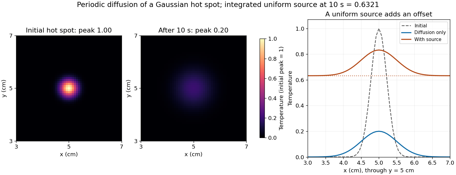
Codex 0 2026-10-25The uniform source adds a background without changing the spatial gradients relative to the unforced solution:At the offset is . On the corrected grid the central peak is therefore about , and regions far from the hot spot are near . The hot spot's broadening is unchanged; the source is spatially uniform. The spatial mean of a periodic heat equation rises by the same amount, tending to a total increment of one temperature unit as .
Past exam of the year 2 of the earth sciences (geology) course of the University of Oxford 2025 Paper 3 7 h Solution by Codex 0 2026-10-25
Codex 0 2026-10-25A spatially uniform source changes only the zero Fourier mode. Its exact integrated increment over a time step beginning at isThe unnormalised two-dimensional discrete Fourier transform stores a constant field as in element This replacement uses the original variable names and MATLAB indexing. The uniform forcing of a periodic heat equation is integrated exactly in time here. No source multiplier is applied to the other modes, and the zero-mode homogeneous multiplier equals one. Adding only
(1,1).[ref]fft2 documentation by MathWorks. The forward defining sum has no normalization; the linked inverse definition includes the factor .
Keep the existing homogeneous exponential multiplication and add this source increment to that element:for i = 1:nt
t = (i-1)*dt;
u_hat = u_hat .* exp(-alpha*K2*dt);
dq = exp(-t/10) - exp(-(t+dt)/10);
u_hat(1,1) = u_hat(1,1) + nx*ny*dq;
enddq to the unnormalised coefficient would underestimate the physical temperature increment by the factor . Past exam of the year 2 of the earth sciences (geology) course of the University of Oxford 2025 Paper 3 7 g Solution by Codex 0 2026-10-25
Codex 0 2026-10-25Aliasing occurs because a sampled grid cannot distinguish certain different continuous Fourier modes. With spacing , modes and agree at every sample point. Frequencies above the Nyquist frequency can therefore be misidentified as lower frequencies, changing the resolved spectrum and its subsequent diffusion rate.
For the corrected grid, and the maximum resolved angular wavenumber is approximately . The initial Gaussian function has spectral envelope proportional to . At that one-coordinate cutoff the factor is about , so the omitted high-frequency tail is tiny. Its continuation mismatch at the distant edges is also tiny. Significant aliasing is not expected for this resolved, smooth initial condition.
The linear constant-coefficient heat equation only damps existing modes; it does not generate higher frequencies through nonlinear products. An unresolved narrow peak, a sharp edge or a nonlinear source would require a separate resolution assessment. The duplicated-endpoint grid issue described above should not be diagnosed as high-frequency folding.
Past exam of the year 2 of the earth sciences (geology) course of the University of Oxford 2025 Paper 3 7 f Solution by Codex 0 2026-10-25
Codex 0 2026-10-25Diffusion smooths and broadens the hot spot while conserving its integral. For an isolated two-dimensional initial profile , the Gaussian hot spot under diffusion isHere and , giving a width parameter of and a peak of in the initial temperature units. The periodic-grid calculation agrees to displayed precision because the periodic copies are far away. Running the endpoint-inclusive listing as written instead gives a sampled initial peak near and final peak near ; the difference is consistent with the coordinate-grid issue, rather than a different diffusion law.
Increasing positive thermal diffusivity at fixed time produces a wider, lower peak. Each nonconstant Fourier mode decays faster, while the spatial mean of a periodic heat equation remains fixed. The profiles approach a uniform mean at long times under these periodic boundary conditions.
Past exam of the year 2 of the earth sciences (geology) course of the University of Oxford 2025 Paper 3 7 e Solution by Codex 0 2026-10-25
Codex 0 2026-10-25- Lines 1–7 set the grid dimensions, domain lengths, thermal diffusivity and time interval. The elapsed time is .
- Lines 9–10 supply coordinates, subject to the periodic-grid correction above. Lines 16–17 sample the initial Gaussian function.
- Lines 11–14 construct the discrete Fourier transform frequency order and . Negative frequencies occupy the second half of each array. This is the discrete version of replacing each spatial derivative by multiplication by .
- Line 20 computes the two-dimensional Fast Fourier transform. Lines 22–24 multiply every mode by at every step, implementing the modal solution derived above.
- Line 26 performs the inverse discrete Fourier transform. Taking the real part removes tiny imaginary roundoff errors; conjugate symmetry of the exact transformed real data already guarantees a real result.
- Lines 28–42 display the initial and final arrays. A common colour scale is needed to compare their peak temperatures; independent automatic colour scales can hide the decrease in amplitude.
For this linear homogeneous problem, the exponential update is exact for the retained modes, apart from roundoff error. It is not a forward Euler method step and does not require the explicit finite-difference diffusion stability restriction. Sampling, periodic modelling and spatial resolution still matter.
Past exam of the year 2 of the earth sciences (geology) course of the University of Oxford 2025 Paper 3 7 d Solution by Codex 0 2026-10-25
Codex 0 2026-10-25- Constant thermal diffusivity makes the Fourier spectral method diagonal: each Fourier mode can be evolved by its exact exponential multiplier.
- The smooth initial Gaussian function has rapidly decaying Fourier coefficients, so a moderate grid resolves it well. The Fast Fourier transform provides an efficient change between the spatial grid and those coefficients.
- A discrete Fourier transform describes a periodically repeated array. Opposite edges are identified by periodic boundary conditions; this is a periodically continued plate model, rather than a plate with prescribed cold or insulated edges.
- The initial hot spot is far from those edges. Over the stated short interval its width remains much smaller than the side length, so the periodic images have negligible influence near the centre. At sufficiently long times, periodic diffusion tends to the conserved spatial mean.
For consistency with the supplied wavenumbers, use an FFT grid on a periodic interval: , , and similarly for . In MATLAB, replace the endpoint-inclusive coordinate definitions by
x = (0:nx-1)*Lx/nx; and y = (0:ny-1)*Ly/ny;. The supplied linspace arrays instead have spacing while the Fourier multipliers assume . Including both copies of the periodic endpoint creates a grid inconsistency, separate from high-frequency aliasing. Past exam of the year 2 of the earth sciences (geology) course of the University of Oxford 2025 Paper 3 7 c Solution by Codex 0 2026-10-25
Codex 0 2026-10-25Let be the Fourier transform of the initial temperature. Solving the scalar linear ordinary differential equation givesRecover using the Fourier inversion theorem, with inverse factor for this two-dimensional convention. Equivalently, take the convolution of the initial data with the two-dimensional heat kernel. On a periodic square, the same exponential applies to each discrete Fourier mode, with and .
Past exam of the year 2 of the earth sciences (geology) course of the University of Oxford 2025 Paper 3 7 b Solution by Codex 0 2026-10-25
Codex 0 2026-10-25Apply the Fourier transform of a derivative twice in each spatial coordinate, and commute the time derivative with the spatial Fourier transform. For the Laplacian,ThusThe minus sign is essential: positive thermal diffusivity damps short spatial scales rather than amplifying them. The zero Fourier mode is unchanged in the absence of a source.
Past exam of the year 2 of the earth sciences (geology) course of the University of Oxford 2025 Paper 3 7 a Solution by Codex 0 2026-10-25
Codex 0 2026-10-25Assume sufficient decay and differentiability to justify integration by parts and exchange of integrals; Schwartz functions are one convenient class. With the stated Fourier transform convention, integrate first in :The boundary contribution vanishes under the decay assumption. The Fourier transform of a derivative consequently turns constant-coefficient spatial differential operators into multipliers. Repeating it gives , so the heat equation becomes an independent temporal ordinary differential equation at each wavevector.
Past exam of the year 2 of the earth sciences (geology) course of the University of Oxford 2025 Paper 3 6 d Solution by Codex 0 2026-10-25
Codex 0 2026-10-25The photic zone is the illuminated layer supporting photosynthesis; its euphotic depth is conventionally associated with about 1% of surface photosynthetically active radiation, integrated over approximately –. This is a useful convention rather than a universal organism-specific compensation depth. Spectral filtering can be represented locally bywhere is the wavelength-dependent diffuse attenuation coefficient. It includes effects of absorption and scattering and is not simply equal to the absorption coefficient .
In clear, low-chlorophyll water, pure water removes red light strongly, while weak blue pigment and CDOM absorption permits blue light, typically around –, to penetrate furthest. The deepest usable light is consequently dim and blue-rich, and the euphotic zone can extend relatively deep. At high pigment concentrations, phytoplankton pigments preferentially remove blue and red light; associated detritus or CDOM can remove still more blue. The remaining transmission window commonly shifts toward blue-green or green wavelengths, roughly –, and the total light falls off faster, so the euphotic depth is shallower. Exact window and depth depend on the full particle/dissolved mixture, not chlorophyll alone. The diagram normalizes the two deep spectra separately to show their different shapes, not equal absolute light at a common depth.
This confines photosynthetic growth to a thinner illuminated interval in high-chlorophyll water and allows a deeper potential habitat in clear low-chlorophyll water, subject also to nutrient supply, mixing and the organism's compensation requirement. Cells near the base benefit from low-light acclimation and pigment systems that capture the remaining wavelengths. In blue-rich deep ocean water, blue-absorbing pigments and some low-light-adapted picoplankton can be favored; where the surviving light is greener, groups with effective green-absorbing accessory pigments, such as certain phycobilins, gain an advantage. A pigment appears coloured by light it fails to absorb, so green-absorbing accessory pigments need not themselves look green. There is no universal deep species determined by chlorophyll concentration alone. A deep chlorophyll maximum can partly reflect increased pigment per cell rather than a proportional maximum in carbon biomass.[ref]
Phytopia's light and color by NASA. Photic-zone discussion: the 1% convention, deep penetration in clear blue waters, and shallower illuminated habitat in productive turbid waters; pigment-based community selection here follows the surviving wavelengths and is conditional.
Past exam of the year 2 of the earth sciences (geology) course of the University of Oxford 2025 Paper 3 6 c Solution by Codex 0 2026-10-25
Codex 0 2026-10-25Chlorophyll a occurs in nearly all oxygen-producing phytoplankton groups and is central to their photosynthesis. Its concentration can be measured reproducibly by pigment extraction or calibrated optical methods, and its absorption affects ocean colour, making it observable over large areas. It is therefore a practical common index of photosynthetic standing stock across diverse communities, unlike a pigment limited to one group.
It is a proxy, not a fixed conversion to phytoplankton biomass or primary production. The carbon-to-chlorophyll ratio varies with species, light acclimation, nutrient supply and physiological condition; low-light cells often contain more pigment per unit carbon. Dead pigment and methodological differences can also affect interpretation, and nonphotosynthetic plankton are not represented. A pigment increase need not mean the same proportional increase in living carbon biomass.[ref]
Chlorophyll maps by NASA Earth Observatory. Chlorophyll alters sunlight absorption and reflection, enabling mapping of near-surface phytoplankton distributions; pigment is used as an index rather than a direct carbon measurement.
Past exam of the year 2 of the earth sciences (geology) course of the University of Oxford 2025 Paper 3 6 b Solution by Codex 0 2026-10-25
Codex 0 2026-10-25Many open-ocean chlorophyll retrieval algorithms infer chlorophyll a from the blue-to-green remote-sensing reflectance ratio. Increasing pigment generally depresses blue reflectance relative to green. In coastal waters, however, coloured dissolved organic matter and non-algal particles can independently absorb blue light, as in the sketches, and therefore mimic an increase in pigment. Their concentrations need not covary with phytoplankton biomass: river runoff and sediment resuspension can change them separately.
Moreover, the satellite measures emerging radiance, not absorption directly. Schematically,where is the backscattering coefficient; this is an explanatory approximation, not a complete retrieval formula. Suspended particles change both absorption and backscattering, and different mixtures can produce similar band ratios. Shallow-bottom reflection, land-adjacency effects and more difficult atmospheric correction introduce further coastal errors. Consequently a simple blue/green ratio can overestimate chlorophyll a when excess CDOM removes blue light, although sediment scattering and other effects mean the bias is not universally positive. Multiband or hyperspectral methods that separately constrain pigment, dissolved absorption and particles, supported by local observations, are preferable in optically complex water.[ref]
Ocean optics protocols by NASA. Revision 4, Volume I: unaccounted blue absorption by CDOM creates regional chlorophyll-retrieval uncertainty; absorption and scattering are distinct optical properties.
Past exam of the year 2 of the earth sciences (geology) course of the University of Oxford 2025 Paper 3 6 a Solution by Codex 0 2026-10-25
Codex 0 2026-10-25The principal non-water visible-light absorbers can be grouped into phytoplankton pigments, coloured dissolved organic matter (CDOM), and non-algal particles (NAP), including organic detritus and absorbing mineral material. A useful additive decomposition of the absorption coefficient isThe supplied sketch separates the three non-water contributions; its amplitudes are arbitrary and are not concentrations or measured spectra.
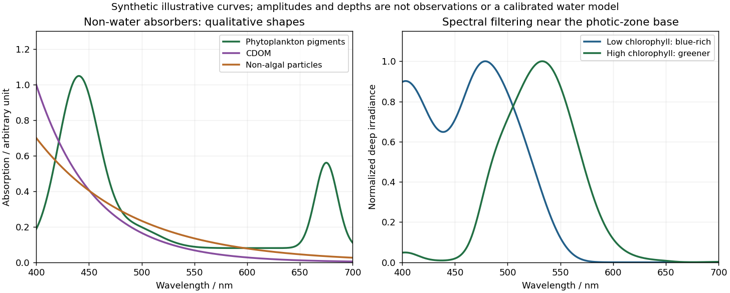
Qualitative marine absorption spectra and deep-light spectral filtering
. Original synthetic sketches: phytoplankton have blue and red pigment absorption bands, while CDOM and non-algal particles preferentially absorb short wavelengths. The right panel illustrates blue-rich deep light in low-chlorophyll clear water and a greener spectrum in more absorbing high-chlorophyll water. Spectra are normalized separately; curves and representative depths are illustrative, not observations or a calibrated radiative-transfer calculation. Details.Phytoplankton pigments give prominent absorption maxima around and , associated with chlorophyll a, and a relative minimum in the green. Accessory pigments, including carotenoids and phycobilins, broaden or add absorption bands, so an assemblage is not just a pure chlorophyll-a solution. Intracellular packaging and cell size also modify the shape and absorption per unit pigment.
Coloured dissolved organic matter consists of dissolved light-absorbing organic compounds, often including humic material from terrestrial runoff and marine degradation. Its absorption is strongest at the blue/ultraviolet end and declines approximately exponentially toward red, without the narrow chlorophyll red peak. A common local parameterization is with positive spectral slope ; here is an optical slope, not gas saturation.
Non-algal particles include nonliving organic detritus, pigment degradation products and absorbing suspended mineral particles. Their aggregate absorption often also decreases approximately exponentially from blue to red, with variable slope and mineral-dependent departures. Suspended sediments can strongly scatter as well as absorb; bright sediment-laden water is not evidence of a red absorption peak. Chlorophyll-containing living cells belong in , so these categories should not be double counted.[ref]
Ocean optics protocols by NASA. Revision 4, Volume I, sections defining chlorophyll, CDOM and non-pigmented-particle absorption, and the importance of blue absorption to ocean-colour retrieval.
Past exam of the year 2 of the earth sciences (geology) course of the University of Oxford 2025 Paper 3 5 b Solution by Codex 0 2026-10-25
Codex 0 2026-10-25Healthy green vegetation has strong visible absorption in the blue, around –, and red, around –, mainly from chlorophylls and other photosynthetic pigments. Weaker absorption around green wavelengths produces a relative reflectance maximum near and the familiar green appearance. The red edge is the steep reflectance rise around –. In the near-infrared, weak pigment absorption and multiple scattering at internal leaf tissue–air interfaces produce high reflectance, commonly a broad plateau. This plateau is primarily a structural scattering effect, rather than chlorophyll reflecting the light.[ref]
Measuring vegetation by NASA Earth Observatory. “Normalized Difference Vegetation Index”: contrast between chlorophyll absorption of visible light and strong near-infrared scattering by leaf structure.
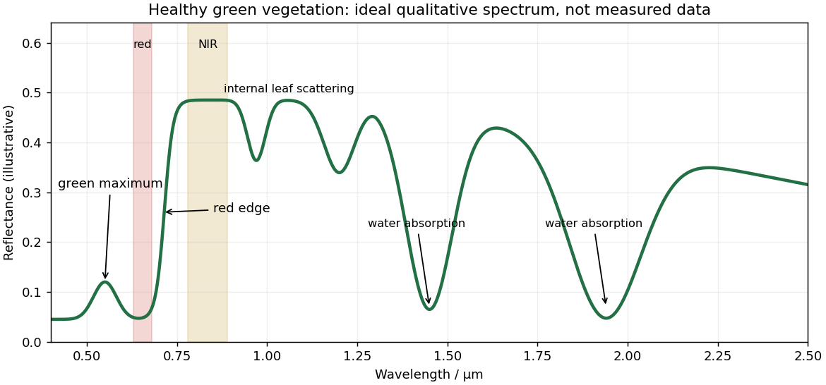
Qualitative reflectance spectrum of healthy green vegetation
. Original synthetic leaf spectrum with a green maximum, red absorption, red edge, near-infrared plateau and shortwave-infrared water absorption troughs. The curve is illustrative rather than measured; shaded bands exemplify red and near-infrared measurements for a vegetation index. Details.Leaf water produces absorption troughs in the shortwave infrared, especially near and , with weaker features near and . Atmospheric water vapor also strongly absorbs near and , so satellite bands usually avoid the centres of those deep troughs. Drying, senescence, pigment loss and changes in canopy structure alter the spectrum; measured canopy reflectance also includes shadows and the soil background.
To highlight vegetation, assign the near-infrared band to the red display channel, red to green and green to blue: vigorously vegetated areas appear bright red in this conventional false-colour composite. Alternatively calculate the normalized difference vegetation index from atmospherically corrected, spatially registered red and near-infrared reflectances:Large positive values indicate a strong vegetation-like red/NIR contrast. For example, and give about . Mask clouds, their shadows and invalid low-signal pixels. Bare soil usually has a smaller contrast, while water often has negative values; fixed universal thresholds are inappropriate, and dense vegetation can saturate the index. A band ratio improves contrast but is not a direct count of plants or a unique measure of physiological health.[ref]
Measuring vegetation by NASA Earth Observatory. “Normalized Difference Vegetation Index”: normalized red/near-infrared contrast and interpretation of green vegetation.
Past exam of the year 2 of the earth sciences (geology) course of the University of Oxford 2025 Paper 3 4 d Solution by Codex 0 2026-10-25
Codex 0 2026-10-25For a surface-breaking reverse earthquake, expect a fault scarp or disrupted belt with the hanging wall displaced upward and commonly over the footwall. Small thrust faults, splays and backthrusts may repeat or override shallow deposits. Shortened soil, roads or other markers may buckle, while soft sediment can form pressure ridges and compression folds. Near the scarp, gravitational collapse and local bending can also produce tensile fissures and small normal faults; a reverse event need not create compression everywhere at the surface.
For a blind reverse rupture, expect coherent uplift and warping, newly tilted surfaces, or a fold scarp without a throughgoing primary fault offset. Small flexural-slip surfaces along bedding, secondary thrust faults or backthrusts, and opening cracks or small normal faults over the bent outer arc of the anticline can accompany the folding. Deformation may be distributed or localized at fold hinges. Thus a blind main fault does not imply an entirely unbroken ground surface, and secondary cracking must be distinguished from the principal rupture by its geometry and displacement pattern. Shaking-triggered landslides or soil liquefaction can accompany either case and should not automatically be mapped as primary tectonic rupture.[ref]
Blind-thrust mapping report by United States Geological Survey. Active fold scarps can arise through localized coseismic uplift and tilting without the principal thrust reaching the ground surface.
Past exam of the year 2 of the earth sciences (geology) course of the University of Oxford 2025 Paper 3 4 c Solution by Codex 0 2026-10-25
Codex 0 2026-10-25Interferometric synthetic-aperture radar compares the phase of coherent radar returns acquired before and after the earthquake from closely repeated viewing geometry. After image registration and removal of orbital and topographic phase, the residual interferometric phase constrains relative ground displacement along the radar line of sight. Defining positive toward the satellite and choosing the interferogram's phase order accordingly,One complete colour cycle therefore represents of relative line-of-sight displacement. Reversing the image order reverses the displayed phase sign. This observes a projection of both horizontal and vertical motion, not uplift alone.[ref]
Interferometry by NASA. NISAR mission explanation: remove orbit/topography contributions and interpret each complete fringe as half a radar wavelength of line-of-sight range change.
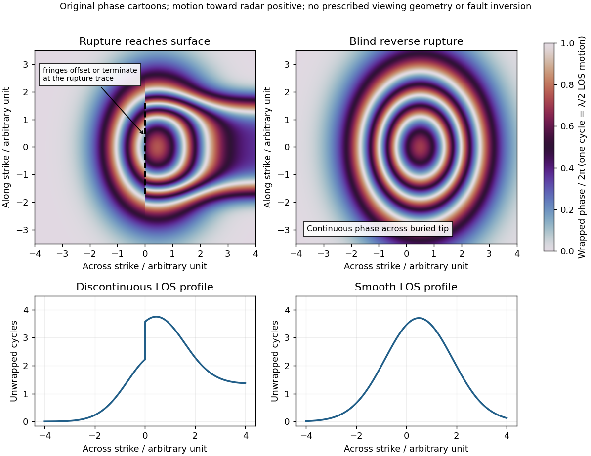
Qualitative interferograms for surface-breaking and blind reverse rupture
. Original wrapped-phase cartoons and corresponding unwrapped line profiles. They illustrate a displacement discontinuity versus a continuous deformation lobe, rather than numerical elastic fault models. The chosen phase sign is positive toward the radar. Every complete colour cycle represents half a radar wavelength of line-of-sight displacement; real fringe shape depends on viewing and rupture geometry. Details.If the main reverse rupture reaches the surface, coherent areas on opposite sides can show a displacement step: fringes become offset, truncated or abruptly juxtaposed along a trace. A narrow belt can lose interferometric coherence where cracking, intense gradients or changed scatterers prevent reliable phase comparison. If the rupture remains blind, a simple elastic model instead predicts a continuous surface displacement field, often a broad asymmetric lobe with continuous curved or closed fringes and a smooth displacement gradient across the projected tip.
These are diagnostic tendencies, not a unique test. An ordinary wrapped-phase boundary is just a colour reset and is not itself a rupture. A step of an integer number of cycles can be hidden in wrapped phase; loss of interferometric coherence can hide either kind of near-field deformation. Vegetation, atmosphere and viewing direction also affect the pattern, and a displacement perpendicular to the radar line of sight is poorly sensed. Inspect coherence and unwrapped displacement, compare ascending and descending views where possible, and test a fault model against field observations. A sharp fold scarp above a blind rupture or a secondary shallow fault can also create localized gradients, so smooth fringes do not prove a buried tip and broken fringes alone do not prove a surface-breaking main rupture.
Pinned article: Introduction to the OurBigBook Project
Welcome to the OurBigBook Project! Our goal is to create the perfect publishing platform for STEM subjects, and get university-level students to write the best free STEM tutorials ever.
Everyone is welcome to create an account and play with the site: ourbigbook.com/go/register. We belive that students themselves can write amazing tutorials, but teachers are welcome too. You can write about anything you want, it doesn't have to be STEM or even educational. Silly test content is very welcome and you won't be penalized in any way. Just keep it legal!
Intro to OurBigBook
. Source. We have two killer features:
- topics: topics group articles by different users with the same title, e.g. here is the topic for the "Fundamental Theorem of Calculus" ourbigbook.com/go/topic/fundamental-theorem-of-calculusArticles of different users are sorted by upvote within each article page. This feature is a bit like:
- a Wikipedia where each user can have their own version of each article
- a Q&A website like Stack Overflow, where multiple people can give their views on a given topic, and the best ones are sorted by upvote. Except you don't need to wait for someone to ask first, and any topic goes, no matter how narrow or broad
This feature makes it possible for readers to find better explanations of any topic created by other writers. And it allows writers to create an explanation in a place that readers might actually find it.
Figure 1. Screenshot of the "Derivative" topic page. View it live at: ourbigbook.com/go/topic/derivativeVideo 2. OurBigBook Web topics demo. Source. - local editing: you can store all your personal knowledge base content locally in a plaintext markup format that can be edited locally and published either:This way you can be sure that even if OurBigBook.com were to go down one day (which we have no plans to do as it is quite cheap to host!), your content will still be perfectly readable as a static site.
- to OurBigBook.com to get awesome multi-user features like topics and likes
- as HTML files to a static website, which you can host yourself for free on many external providers like GitHub Pages, and remain in full control

Figure 2. You can publish local OurBigBook lightweight markup files to either OurBigBook.com or as a static website.
Figure 3. Visual Studio Code extension installation.
Figure 5. . You can also edit articles on the Web editor without installing anything locally. Video 3. Edit locally and publish demo. Source. This shows editing OurBigBook Markup and publishing it using the Visual Studio Code extension. 
- Infinitely deep tables of contents:




All our software is open source and hosted at: github.com/ourbigbook/ourbigbook
Further documentation can be found at: docs.ourbigbook.com
Feel free to reach our to us for any help or suggestions: docs.ourbigbook.com/#contact