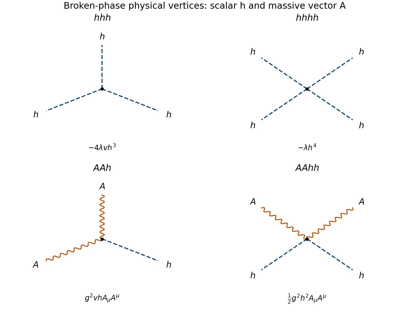
A real antisymmetric generator of the connected rotation group isChoose $D_{\mu }\mathbf{\varphi }=({\partial }_{\mu }-g{A}_{\mu }T)\mathbf{\varphi }$. Under $\mathbf{\varphi }\mapsto R(\alpha (x))\mathbf{\varphi }$ and $A_{\mu }\mapsto A_{\mu }+{\partial }_{\mu }\alpha /g$, the gauge covariant derivative transforms in the same way as the field. Include the canonical gauge kinetic term $-F_{\mu \nu }{F}^{\mu \nu }/4$ so the vector's mass normalization is specified.

In unitary gauge, $\mathbf{\varphi }=(v+h,0{)}^T$. The relevant Lagrangian density isReading the quadratic vector term as $m_A^2{A}^2/2$ givesThe angular scalar supplies the longitudinal polarization of the massive vector; it is not a separate physical massless particle after gauging. The physical scalar still has $m_h^2=8\lambda v^2$.

The interactions among the physical fields areThus the complete physical vertex list is $hhh$, $hhhh$, $AAh$, and $AAhh$. An Abelian gauge kinetic term generates no $AAA$ or $AAAA$ self-interaction. Gauge-dependent Goldstone vertices in another gauge do not add physical particle species to this list. These statements concern the broken phase $v\ne 0$; when $v=0$ the unitary-gauge broken-phase parametrization is unavailable.

At an arbitrary nonzero vacuum write ${\mathbf{\varphi }}_{\ast }=|v|\mathbf{n}$, where ${\mathbf{n}}^T\mathbf{n}=1$. The Hessian matrix of the potential isOn the vacuum circle this reduces toIt has eigenvalue $8\lambda v^2$ along $\mathbf{n}$ and eigenvalue zero along the one perpendicular direction. Rotating the vacuum conjugates this matrix by an orthogonal matrix and cannot change its eigenvalues. Thus every point on the circle has exactly one tangential massless Goldstone boson.

Geometrically, motion along the circle costs no potential energy whereas motion normal to it does. The circle's dimension, equivalently $\dim O(2)-\dim O(1)=1$, is independent of its point. Counting the number of real field components would instead give two and would incorrectly count the massive radial direction as a Goldstone mode.

Any constant real orthogonal matrix $R$ acting by $\mathbf{\varphi }\mapsto R\mathbf{\varphi }$ preserves both the Euclidean field-space norm and the kinetic term. The full internal symmetry is $O(2)$, with connected component $SO(2)\simeq U(1)$; reflections add a discrete component.

For $v\ne 0$, the vacuum manifold is the circle ${\mathbf{\varphi }}^T\mathbf{\varphi }=v^2$. Expand about the chosen point as ${\varphi }_1=v+h$, ${\varphi }_2=\pi$. The potential becomesThe kinetic terms remain canonically normalized real-scalar kinetic terms. Comparing the quadratic potential with $m_h^2{h}^2/2+m_{\pi }^2{\pi }^2/2$ givesThere is one massive radial mode and one massless tangential Goldstone boson. A chosen vacuum leaves only the reflection that fixes that point, so there is one broken continuous generator. For negative $v$ the chosen point lies on the opposite side of the same circle and the mass depends on $v^2$; the radius is $|v|$. If $v=0$, the vacuum circle collapses to the origin, no continuous generator is broken, and both quadratic masses vanish without either field being a Goldstone mode. The nonzero-$v$ assumption is essential to the spontaneous-breaking interpretation.

With the Minkowski metric $(+---)$, the momentum conjugate to the real field vector is $\mathbf{\pi }=\dot{\mathbf{\varphi }}$. The Hamiltonian density isAssume the potential has a global minimum $V_{\min }$ and the boundary conditions permit a constant minimizing field. ThenThe bound is attained byThe homogeneous vacuum minimum criterion proves existence of a homogeneous lowest-energy configuration under those assumptions. On infinite space one subtracts the constant vacuum energy before comparing finite energy differences. This identifies the classical vacuum configuration; it does not assert that the quantum field has no fluctuations.

The claim does not follow from “no derivative dependence in $V$” alone. For example, the allowed functional form $V(\varphi )=-{\varphi }^4$ is unbounded below, so there is no state of lowest energy to identify. Boundary conditions forcing different vacua at opposite ends can instead require an inhomogeneous minimum, such as a domain wall. The positive quartic potential used in the following parts does have homogeneous minima, so these caveats do not obstruct its vacuum calculation.

At $B=0$ a global reversal ${\sigma }_j\mapsto -{\sigma }_j$ leaves the energy and statistical weight unchanged but changes the sign of the one-spin observable. Pairing reversed configurations givesEquivalently, $⟨\pm |{\sigma }^z|\pm ⟩=0$ in the transfer eigenbasis, so $\mathrm{Tr}({\sigma }^z{T}^N)=0$. This holds for every finite even ring and all finite temperatures, and for the zero-field Gibbs limit. A symmetry-selected zero-temperature alternating state can have nonzero staggered magnetization; its uniform magnetization is still zero. The classical spin variable in this model has no separate quantum spin-operator dynamics despite the conventional matrix notation ${\sigma }^z$ used for the insertion.

At zero field the normalized transfer matrix for a classical spin chain eigenvectors and eigenvalues areThe spin insertion exchanges the two eigenvectors: ${\sigma }^z|+⟩=|-⟩$ and conversely. Evaluating the trace in c therefore gives, with $x={\lambda }_{-}/{\lambda }_{+}=-\tanh K$,This is the finite-ring result. In the thermodynamic limit, or for $1\ll r\ll N$ away from the wrap-around image, it becomesHere $\xi$ is in lattice-site units. The alternating sign is antiferromagnetic order at short distances; the exponential envelope shows the absence of long-range order at every positive temperature in this one-dimensional finite-range model. As $T\to 0$, $\xi$ diverges, asymptotically $\xi \sim \frac{1}{2}{e}^{2\beta J}$. For the even ring the zero-temperature result is $g(r)=(-1{)}^r$, consistent with the two alternating ground configurations. At fixed finite $N$, “large distance” must still respect periodicity: $g_N(r)=g_N(N-r)$ rather than decaying indefinitely beyond the ring.

Insert the two observed spins into the configuration sum for the transfer matrix for a classical spin chain trace. Since the diagonal matrix ${\sigma }^z$ has entry $s$ on state $s$, multiplication by it at positions $j$ and $j+r$ produces the factor ${\sigma }_j{\sigma }_{j+r}$. The trace representation is consequentlyThere are exactly $N$ transfer factors: $(j-1)+r+(N+1-j-r)=N$. The distance between the two insertions is $r$ bonds, not $r-1$. Cyclicity of the trace combines the outside factors and gives the equivalent expressionwhich makes independence of the starting site manifest. No assumption that $T$ commutes with ${\sigma }^z$ is used; in general it does not. For $r=0$ the two insertions multiply to the identity and $g(0)=1$, a useful normalization check.

Share each on-site field energy equally between its two neighboring bonds. In the ordered basis $\sigma =+1,-1$, the symmetric transfer matrix for a classical spin chain isThe product ${\prod }_j{T}_{{\sigma }_j{\sigma }_{j+1}}$ recovers each bond and each field term once. Summing the periodic indices closes a trace, giving $Z_N=\mathrm{Tr}{T}^N$. The two eigenvalues areThe square-root argument is positive. Moreover $\det T=e^{-2K}-e^{2K}<0$, so ${\lambda }_{-}<0$ even at nonzero field. Its sign must not be discarded merely because all matrix entries are positive. The Perron–Frobenius theorem ensures that the positive eigenvalue ${\lambda }_{+}$ has the larger modulus, and the infinite-chain free energy is $f_{\infty }=-{\beta }^{-1}\log {\lambda }_{+}$. For even $N$, both terms in the finite-size partition function are positive.

Let $\beta =(k_{B}T{)}^{-1}$, and sum over all $2^N$ configurations satisfying the periodic identification. The canonical partition function and finite-size free energy per site areThe plus sign multiplying $J$ in the energy means that $J>0$ favors opposite neighboring spins: this is an antiferromagnetic Ising model. Even $N$ permits an alternating configuration to close without frustration. The finite-size formula does not require taking a thermodynamic limit; that limit is taken only after evaluating $Z_N$.

Specify the Fourier transform before performing the Gaussian integral:At $u=0$ the functional is diagonal in both component and momentum, with inverse kernels $q^2+t+r$, $q^2+t-r$, and $q^2+t$. The condition $0<r<t$ makes all three positive. The covariance of a Gaussian distribution with statistical weight $e^{-F/(k_{B}T)}$ is $k_{B}T$ times the inverse kernel, henceIf $F$ is already the dimensionless free energy divided by $k_{B}T$, the numerators are one instead. Translational invariance forces opposite momenta to pair. There is no complex conjugate on the second field, so the delta function is at $\mathbf{p}=-\mathbf{q}$, not at $\mathbf{p}=\mathbf{q}$. A correlation with $m_j(\mathbf{p}{)}^{\ast }$ would have the latter convention. Rotational symmetry in real space leaves dependence on $q^2$ alone once the momentum-conservation delta function is factored out. The correlation lengths are ${\xi }_1=(t+r{)}^{-1/2}$ and ${\xi }_2=(t-r{)}^{-1/2}$; the second component becomes soft as $r\uparrow t$. The skipped letter in the source is preserved: this solution is part (e), with no inferred part (d).

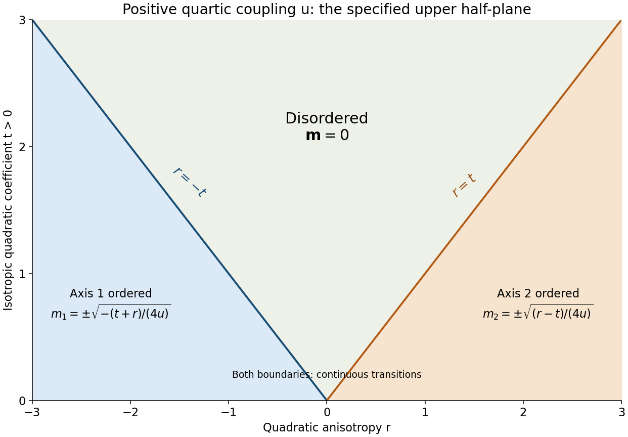
Assume $u>0$, as required for the stable quartic model, and retain the stated domain $t>0$. For the opposite-axis quadratic anisotropy of a vector order parameter, fix the magnitude $\rho$. Then the anisotropy lowers the energy most by putting all magnetization along component 1 if $r<0$ and component 2 if $r>0$. Component 3 has positive quadratic coefficient $t$ and cannot lower the uniform minimum. Minimizing the remaining amplitude givesThe component-1 and component-2 ordered regions each break a discrete sign symmetry, giving two easy-axis orientations rather than a sphere of equivalent directions. To check stability, in the component-1 minimum the longitudinal curvature is $-2(t+r)>0$, while the two transverse curvatures are $-2r>0$ and $-r>0$. The component-2 case similarly has longitudinal curvature $-2(t-r)$ and transverse curvatures $2r,r$, all positive in its region. The disordered state is stable exactly when $t\pm r\ge 0$.

Both boundaries $r=-t$ and $r=t$ are continuous, second-order mean-field transitions: the selected component vanishes with a square root, and the first derivatives of the minimum free energy agree across the boundary. In the stipulated upper half-plane $t>0$, the two ordered phases are separated by a disordered wedge. There is no direct first-order boundary between them in that domain. Extrapolating a phase boundary through $t<0$ would answer a different, larger phase-diagram question.

Vary each field component independently and integrate the gradient term by parts, taking fixed boundary values or vanishing surface variations. With $\rho =m_1^2+m_2^2+m_3^2$, the Euler-Lagrange equations for the free-energy saddle areThe anisotropy shifts the first two inverse susceptibilities in opposite directions. The derivative of $u{\rho }^2$ is $4u\rho m_j$, which fixes the factor needed for both the magnetization and the free energies in c. Under natural free-boundary conditions the integration by parts instead supplies ${\partial }_n{m}_j=0$ at the surface.

For an analytic, local Landau theory with independent global rotations of the magnetization vector, a uniform scalar potential can depend only on $\rho =\mathbf{m}\cdot \mathbf{m}$. Keeping terms through fourth order in the field, dropping an additive constant, and retaining the leading isotropic positive gradient term gives the displayed quadratic-plus-quartic functional. The stiffness has been absorbed into the normalization of length and field. Higher powers and higher derivatives are neglected in this long-wavelength approximation.

The quartic truncation is stable at large $|\mathbf{m}|$ when $u>0$. The coefficient $t$ changes sign at the mean-field critical point; close to it one commonly writes $t\propto T-T_c$. If $u<0$, higher stabilizing powers are essential, so the displayed truncation alone cannot determine a stable first-order phase diagram. For $u=0$ and $t<0$ it is likewise unbounded.

For $u>0$, spatially uniform stationary points obey $(t+4u\rho )\mathbf{m}=0$. The global minima areThe corresponding minimum free-energy density is zero and $-t^2/(16u)$, respectively. The disordered phase gives way continuously to a ferromagnet with an arbitrary direction of magnetization. At this mean-field transition the amplitude vanishes as $(-t{)}^{1/2}$; long-wavelength critical fluctuations can modify mean-field exponents in three dimensions.^[ref]

Choose the positive-$x$ polarized ground state selected by $B>0$, or its symmetry-selected $B\to 0^{+}$ limit. It is exactly the boson vacuum in the Holstein–Primakoff transformation. Thus $n_j|\mathrm{GS}⟩=0$ and $S_j^x=S-n_j$ giveFor the transverse components, $S^y=({\tilde{S}}^{+}+{\tilde{S}}^{-})/2$ and $S^z=({\tilde{S}}^{+}-{\tilde{S}}^{-})/(2i)$. In the vacuum, the only nonzero quadratic ladder-operator expectation iswhich follows using the full ordered square-root operators, or directly from ${\tilde{S}}^{-}|S,S⟩=\sqrt{2S}|S,S-1⟩$. ThereforeAn independent exact spin argument starts from $S_j^x|S,S{⟩}_x=S|S,S{⟩}_x$ and $(S_j^x{)}^2+(S_j^y{)}^2+(S_j^z{)}^2=S(S+1)$. Rotational invariance about $x$ makes the two transverse second moments equal, so each is $[S(S+1)-S^2]/2=S/2$. This agrees exactly with the full boson representation.

The first moments describe the local magnetization. Subtracting their squares from the second moments gives spin component variances: zero longitudinal variance and transverse variance $S/2$. Transverse quantum fluctuations persist in a perfectly polarized state even though its magnon occupation is zero. Their relative scale decreases as $S^{-1/2}$ in the classical limit.

At precisely $B=0$, “the ground state” requires a choice within the ferromagnetic multiplet. For example, when $NS$ is an integer, a maximum-total-spin state with total $x$ projection zero is also a ground state but has $⟨S_j^x⟩=0$. The displayed local moments refer to the explicitly specified polarized member, not to every superposition or rotationally invariant mixture of zero-field ground states.

Quantize along the selected field direction by the right-handed relabeling ${\tilde{S}}^z=S^x$, ${\tilde{S}}^x=S^y$, ${\tilde{S}}^y=S^z$. Then the exact Holstein–Primakoff transformation in c gives $S_j^x=S-n_j$. Keep exchange terms of order $S^2$ and $S$, with $J$ and the printed $B$ held fixed. For a nearest-neighbor bond,On a periodic cubic lattice with $N$ sites and spacing $a$, there are $3N$ undirected bonds. Consequently,Use the unitary lattice Fourier transform $a_j=N^{-1/2}{\sum }_{\mathbf{k}}{e}^{i\mathbf{k}\cdot {\mathbf{r}}_j}{a}_{\mathbf{k}}$. Each positive lattice direction contributes $2(1-\cos k_{\alpha }a)$, so the Hamiltonian operator is already diagonal in momentum space:There are no anomalous $aa$ or $a^{†}{a}^{†}$ terms, so no Bogoliubov transformation or extra zero-point correction is needed. At long wavelengths,At $B=0$ this is the quadratic ferromagnetic Goldstone mode; for $B>0$ it is gapped by $BS$. Energies are written with $\hslash =1$; an excitation frequency is ${\omega }_{\mathbf{k}}={\epsilon }_{\mathbf{k}}/\hslash$. In this isotropic ferromagnet the fully aligned vacuum and its one-magnon dispersion are also exact; higher-magnon interactions are among the terms discarded from the linear spin-wave Hamiltonian operator.

For a local spin quantized along its positive $\tilde{z}$ axis, the exact Holstein–Primakoff transformation isThe bosonic operators obey $[a_j,a_k^{†}]={\delta }_{jk}$. The physical local subspace is $0\le n_j\le 2S$; the larger unconstrained boson Fock space is not itself the finite spin Hilbert space. The ordering of the square roots matters, since $n_j$ does not commute with $a_j$.

This represents spin lowering using a bosonic creation operator, making a fully polarized spin state the boson vacuum. On the physical subspace it reproduces the spin commutators and the Casimir ${\tilde{\mathbf{S}}}_j^2=S(S+1)$. Expanding the square roots for small occupation relative to $S$ organizes a controlled large-$S$ linear spin-wave approximation; it is not an assumption that a spin has an infinite number of physical levels.

The field term explicitly selects the positive $x$ direction. For $B>0$ the uniform minimizing state is ${\mathbf{S}}_j=S\hat{\mathbf{x}}$, with no remaining continuous degeneracy of its orientation. Rotations about the $x$ axis still leave the Hamiltonian operator invariant, and the selected state respects that residual symmetry.

Tilting the magnetization now costs a field energy. Accordingly the transverse spin wave acquires a gapas confirmed directly in d. The factor $S$ is present because the source couples the field as $-BS{\sum }_j{S}_j^x$ rather than $-B{\sum }_j{S}_j^x$. Gapless zero-field Goldstone modes need not survive an explicit symmetry-breaking field.

The negative sign of the exchange term and $J>0$ make this a Heisenberg ferromagnet. Each classical bond minimizes its energy when its two fixed-length spins are parallel. On the connected cubic lattice all ground states are therefore uniform:using length $S$ for the classical large-spin convention. Any two orientations are related by a common spatial rotation of every spin. The global spin-rotation symmetry is $SO(3)$, and a chosen direction retains its $SO(2)$ subgroup of rotations about that axis.

Spontaneous symmetry breaking means selecting one member of this continuous set in the thermodynamic limit, for example by taking volume to infinity before sending an aligning field to zero. The zero-field Hamiltonian operator remains rotationally invariant even though the selected state is not. There are gapless transverse spin waves. Although two rotation generators are broken, an isotropic ferromagnet has one quadratic magnon branch, whose two transverse spin components form a conjugate dynamical pair. It is not necessary to invent two independent linear-dispersion branches from the number of broken generators. The long-wavelength dispersion is derived in d.

For equal rates, the master equation generator is $f$ times the symmetric path-graph matrixIts eigenvectors may be chosen as $(1,1,1)$, $(1,0,-1)$, and $(1,-2,1)$, with eigenvalues $0,-f,-3f$. Resolve the initial empty state asEach nonstationary eigencomponent decays with its own rate, givingThe remaining probabilities are $p_0(t)=1/3+e^{-ft}/2+e^{-3ft}/6$ and $p_A(t)=(1-e^{-3ft})/3$. These satisfy the full equations and sum to one. The limit $p_B(\infty )=1/3$ agrees with the stationary result. At short times $p_B(t)=f^2{t}^2/2+O(t^3)$: two successive jumps, $0\to A\to B$, are necessary, so a term linear in $t$ would signal an incorrectly included direct transition.