A stationary evanescent wave does not assign a classical trajectory or a real local speed inside the forbidden region. The dwell time in a semi-infinite potential step measures probability stored in $x>0$ divided by incident probability current. For incident amplitude one,This gives a time in terms of $m,E,V_0$ through the definitions of $k,\kappa$. A simpler dimensional estimate is the penetration length divided by the incident speed, $\Delta x/v_{\mathrm{in}}=m/(\hslash k\kappa )=\hslash /[2\sqrt{E(V_0-E)}]$. The dwell time equals $(2E/V_0)$ times that estimate. Different operational timing definitions need not agree; treating the imaginary under-barrier momentum as a real particle velocity would not justify a unique traversal time.

The wave-function amplitude decays as $e^{-\kappa x}$, so its e-folding penetration depth isThe probability density decays as $e^{-2\kappa x}$ and has the smaller e-folding depth $1/(2\kappa )$. Specifying which quantity decays avoids a factor-of-two ambiguity in the term penetration depth.

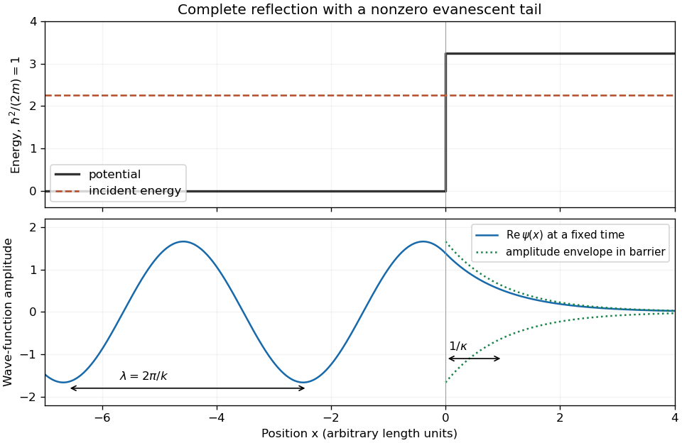
On the incident side, $\varphi$ is the superposition of incoming and reflected waves, producing a standing-wave pattern whose travelling-wave de Broglie wavelength is $\lambda =2\pi /k$. On the forbidden side, it decays exponentially and remains nonzero near the boundary. A sketch should therefore show oscillations for $x<0$, a continuous function and slope at zero, and the evanescent tail for $x>0$ beside the potential step.

The quantum distinction is finite probability density inside the classically forbidden region, despite complete reflection. There is no transmitted flux at arbitrarily large positive $x$ for this semi-infinite step. A finite-width barrier would allow quantum tunnelling, a different boundary-value problem.

The reflection-one result describes a semi-infinite potential step, rather than a finite-width barrier. Define $k=\sqrt{2mE}/\hslash$ and $\kappa =\sqrt{2m(V_0-E)}/\hslash$. For $E>0$, takeThe growing exponential is excluded by boundedness as $x\to \infty$. Continuity of $\varphi$ and ${\varphi }^{\prime }$ at the finite step gives $1+r=c$ and $ik(1-r)=-\kappa c$, henceThe probability current of the decaying tail is zero; the reflected and incident currents have equal magnitude. This agrees with the classical reflection coefficient even though the spatial wave function differs from a classical trajectory.

The one-dimensional Time-dependent Schrödinger equation isThe left side generates time evolution; the two terms on the right are the kinetic and potential parts of the Hamiltonian operator. For a time-independent potential and an energy eigenstate, set $\psi (x,t)=\varphi (x)e^{-iEt/\hslash }$. Cancelling the time factor gives the time-independent Schrödinger equation, $-{\hslash }^2{\varphi }^{\prime \prime }/(2m)+V\varphi =E\varphi$.

By the Born rule, $|\psi {|}^{2}dx$ is the position probability in an interval of width $dx$, with $\int |\psi {|}^{2}dx=1$ for a normalized particle. Therefore $\boxed{[\psi ]={\mathrm{length}}^{-1/2}}$ in one dimension. An ideal scattering plane wave instead uses flux normalization and is not itself a normalizable single-particle state on the whole line.

Within an already specified inertial frame, with constant mass, substituting zero resultant force into Newton's second law does give zero acceleration. In that limited mathematical sense, force-free uniform motion is a special case. The reason for retaining Newton's first law is that its physical role is broader than this substitution.

The second law does not, just by its algebra, identify the coordinate systems in which acceleration measures the response to physical interactions. A free body described in coordinates $x^{\prime }=x-\frac{1}{2}A{t}^2$ has ${\ddot{x}}^{\prime }=-A$, despite experiencing no impressed interaction. If the second law is restricted to inertial frames, the first law supplies a criterion for that restriction and asserts that a common inertial structure exists. If instead one introduces a fictitious force $-mA$ to preserve the equation in the accelerated coordinates, that coordinate-dependent bookkeeping should not be confused with a newly discovered physical interaction.

Nor can the first law simply be used as a circular definition in which “free” means “unaccelerated” and “inertial” means “whatever makes the chosen body free”. The framework requires empirical identification of interactions and a mutually consistent class of free-body trajectories. Removing an influence or improving isolation should make the same inertial description work for many bodies, not merely one fitted trajectory.

Thus the two laws have distinguishable jobs: the first articulates the force-free inertial background; the second quantifies departures caused by impressed forces. A modern axiomatization may build that background into its spacetime structure and then omit a separately numbered first law. That is a legitimate reorganization, but it incorporates the first law's content rather than obtaining all of it from the equation $\mathbf{F}=m\mathbf{a}$. Newton states the laws separately in the opening axioms.^[ref]

Showing that acceleration is unchanged by a uniform boost is necessary, but it is not enough to establish the Galilean covariance of Newton's second law. One must specify how time, positions, masses, forces and any background physical systems transform, and show that the actual force laws retain their form.

For a constant spatial rotation $R$, boost velocity $\mathbf{U}$ and translations, writeDifferentiation gives ${\mathbf{v}}^{\prime }=R\mathbf{v}-\mathbf{U}$ and ${\mathbf{a}}^{\prime }=R\mathbf{a}$. Assuming invariant inertial mass,Consequently the equation has the same form if the resultant physical force satisfies ${\mathbf{F}}^{\prime }=R\mathbf{F}$. For a pure boost, this reduces to ${\mathbf{F}}^{\prime }=\mathbf{F}$. More explicitly, if a force is represented by a function of positions, velocities and other physical data, those arguments and data must transform so that its primed value is $R$ times the old value. It is this condition on the complete dynamical model, not the typography of $\mathbf{F}=m\mathbf{a}$, that establishes covariance.

An instantaneous inverse-square interaction depending on the separation of two particles passes this test: their common boost cancels from the separation, and a rotation rotates the force vector. A resistance law $\mathbf{F}=-\zeta (\mathbf{v}-\mathbf{u})$ also passes when the medium's velocity $\mathbf{u}$ transforms with the body. In contrast, keeping $\mathbf{F}=-\zeta \mathbf{v}$ in every boosted frame while silently resetting the same medium to rest changes the physical problem. That model has not been shown covariant by noting ${\mathbf{a}}^{\prime }=\mathbf{a}$.

Likewise, the full Maxwell equations are not made Galilean covariant merely because some equation of particle motion is written as force equals mass times acceleration. The covariance of a framework has to be checked together with its interaction laws. Newton's own Corollary V expresses the corresponding equivalence of uniformly translating, nonrotating systems for the mechanics under consideration.^[ref]

Newton's first law says that a body retains uniform rectilinear motion, including rest as the zero-velocity case, unless impressed forces change that motion. Its physical content includes the existence of a common class of inertial frames: free bodies do not each require an unrelated frame chosen just to straighten their own trajectory. Uniformity refers to the inertial time parameter, and straightness to the spatial structure of those frames. Everyday slowing under friction is compatible with this claim because it involves an interaction, not an exception to inertia.

Newton's second law relates the impressed resultant force to change of momentum. In modern continuous-force notation,so for constant mass it becomes $m\mathbf{a}={\mathbf{F}}_{\mathrm{net}}$. An impulsive version is $\Delta \mathbf{p}=\int \mathbf{F}dt$. The change is directed along the impressed resultant, not necessarily along the body's current velocity. The original wording concerns change of quantity of motion; the differential equation is its modern continuous-time formulation.^[ref]

These are substantive physical claims only when mass, interactions and the inertial structure are constrained independently. If “force” merely abbreviates whatever equals $m\mathbf{a}$ in any arbitrarily chosen coordinates, the second law by itself predicts nothing. Actual applications combine the law with independently testable interaction laws, vector addition of forces, initial conditions and a specification of the inertial frames.

Let $Q$ be annual emissions abatement in tonnes per year. The given marginal abatement cost isUnder the stipulated global, stationary, unconstrained cost-benefit model, the optimal interior abatement equates that marginal cost to the avoided marginal damage of approximately $166.7\mathrm{USD}$ per tonne. ThusTotal mitigation expenditure is the area under the marginal-cost curve, not its endpoint value times all abated tonnes:The result also presumes baseline emissions permit this much reduction. Rational policy need not reproduce it: different discounting, damage uncertainty and risk aversion, income weights, omitted ecosystem impacts, adaptation and local air-quality benefits alter valued benefits; technology learning and adjustment constraints alter costs. Separate rational governments may abate less because some benefits accrue abroad, while cooperative policy can internalize those benefits. Future climate or technology changes also undermine a fixed present marginal-damage curve. These are changes in the optimization problem, not evidence of irrational decision-makers.

Insert the pulse response into $D=\beta (T-T_0)$ and write $u=t^{\prime }-t_e$. For a positive discount rate $k_D$,ThereforeWith $k_D=0.03\mathrm{yea}{\mathrm{r}}^{-1}$, $k_T=0.05\mathrm{yea}{\mathrm{r}}^{-1}$ and the supplied one-tonne normalization of $A$,This is valued at the time of emission because the discount factor is relative to that date. Valuing an emission at a future date from an earlier reference date would require an additional discount factor. The infinite-horizon integral converges for $k_D>0$ under the assumed persistent forcing.

For logarithmic forcing $F=a\ln (C_a/C_{a0})$, where $C_a$ denotes atmospheric carbon-dioxide concentration rather than heat capacity, $\dot{F}=(a/C_a){\dot{C}}_a$. Approximately constant $\alpha$ in $\dot{F}=\alpha E$ therefore requires a roughly constant conversion from emissions to persistent atmospheric burden and a concentration range small enough to hold $a/C_a$ fixed. Carbon removal must be negligible on the modeled horizon, or be replaced by a fixed retained fraction; a realistic multiscale carbon-cycle response generally violates the permanent-step approximation.

A one-tonne pulse at time $t_e$ is $E(t)=\delta (t-t_e)$ in tonne-normalized units. It gives a persistent forcing step $F=\alpha \Theta (t-t_e)$. Convolving that step with the thermal response yieldsThere is no instantaneous temperature jump for finite $C$, although forcing jumps. Both persistence and constant coefficients are deliberate simplifications, rather than an assertion that all emitted carbon dioxide remains airborne forever.

Put $\vartheta =T-T_0$ and assume $C>0$, $\lambda >0$. The linear differential equation for a constant forcing step isMultiplying by the integrating factor $e^{\lambda t/C}$ and integrating from zero to $t$ givesThe response initially grows at rate $F_0/C$ and tends to the equilibrium warming $F_0/\lambda$. Heat capacity per unit area and radiative-feedback units make $k_T$ an inverse time.

The quadratic coefficient must have units $\mathrm{W}{\mathrm{m}}^{-2}{\mathrm{K}}^{-2}$; the printed ${\mathrm{K}}^{-1}$ makes its term dimensionally incompatible with a radiative flux. Interpret its numerical value as ${\lambda }_2=0.05\mathrm{W}{\mathrm{m}}^{-2}{\mathrm{K}}^{-2}$, with ${\lambda }_1=1.5\mathrm{W}{\mathrm{m}}^{-2}{\mathrm{K}}^{-1}$. The total imbalance isA quadrupling gives $F_{\mathrm{ext}}=2(3.75)=7.5\mathrm{W}{\mathrm{m}}^{-2}$. The two equilibrium roots areFor positive heat capacity, stability requires $\partial N/\partial T=-{\lambda }_1+2{\lambda }_2\Delta T<0$. Thus only the lower root is stable. A saddle-node bifurcation occurs atThe logarithmic forcing relation gives $C_{\mathrm{crit}}=2802^{11.25/3.75}=2240\mathrm{ppm}$. Strict linear stability holds below this concentration on the lower branch; the equality is marginal and is the supremum, not another strictly stable equilibrium. Sustained forcing above it causes warming without a balancing equilibrium in this quadratic model. At such large changes its local feedback expansion can fail, and other physics can intervene; it does not prove unlimited real-planet warming or locate a measured Earth runaway threshold.

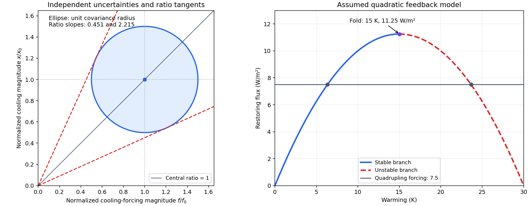
Take the logarithmic forcing law with its normalization fixed by the given doubling value. Let $x$ be the positive magnitude of cooling and $f$ the positive magnitude of the earlier negative forcing:At $C=212\mathrm{ppm}$, $f_0=1.5051\mathrm{W}{\mathrm{m}}^{-2}$. Equilibrium then yieldsThe concentration endpoints $185$ and $244\mathrm{ppm}$ imply forcing magnitudes $2.242$ and $0.7445\mathrm{W}{\mathrm{m}}^{-2}$, approximately $f_0\pm 0.75$. Define normalized variables $u=f/f_0$ and $v=x/x_0$. Independent approximately Gaussian uncertainties give the one-standard-deviation covariance ellipseIts centre is $(1,1)$ and its principal directions are the two coordinate axes. Warming is $2.492(v/u)\mathrm{K}$, so rays from the origin have constant inferred warming. The bounding rays tangent to this ellipse have slopes $m$ satisfying $(1-m{)}^2=\frac{1}{4}(1+m^2)$, orThis gives the useful asymmetric one-parameter profile estimateThe concentration data supply only marginal intervals, not a full likelihood. This result explicitly approximates their logarithmic forcing uncertainty as Gaussian. Linear error propagation would instead give fractional uncertainty $\sqrt{0.5^2+0.5^2}=0.707$, or roughly $2.49\pm 1.76\mathrm{K}$, and misses the large reciprocal asymmetry. A unit-radius two-dimensional covariance ellipse itself contains about $39\%$ of a bivariate Gaussian, not $68\%$; the quoted interval uses the one-parameter $\Delta {\chi }^2=1$ profile/ratio construction, rather than claiming that ellipse is a $68\%$ joint region.

Use a positive stabilizing feedback coefficient: the net flux is $N=F_{\mathrm{ext}}-\lambda \Delta T$. The Planck feedback increases outgoing thermal radiation as temperature rises and therefore contributes positively to $\lambda$. Water-vapor feedback raises infrared opacity as a warmer atmosphere holds more water, tending to reduce $\lambda$; ice-albedo feedback also tends to reduce it as bright ice is lost. These signs depend on the explicitly stated convention.

For doubled carbon dioxide forcing $F_{2\times }>0$, equilibrium givesA symmetric positive interval $[{\lambda }_0-{\sigma }_{\lambda },{\lambda }_0+{\sigma }_{\lambda }]$ maps toThe upward excursion is larger than the downward one because inversion is nonlinear. If the interval reaches zero, it supplies no finite upper bound on equilibrium warming within this linear stable model.

The actual Earth response to doubling carbon dioxide is expected to be much smaller than this roughly $60\mathrm{K}$ all-grey-absorbers estimate. Carbon dioxide absorbs in selected spectral bands rather than doubling opacity across the entire thermal spectrum, and doubling it does not double the other infrared absorbers. Saturated band centres and overlap with water absorption further distinguish it from uniform opacity multiplication. Changes in water vapour, clouds and the lapse rate introduce important climate feedbacks, but do not justify treating the real atmosphere as the stipulated dry, wavelength-independent absorber. The idealized number is therefore not an estimate of real-world equilibrium climate sensitivity.

Let $q$ be the mass mixing ratio of the uniformly mixed infrared absorbers, and let $k$ be their constant mass absorption coefficient. Hydrostatic integration gives downward optical depth $\tau =kqp/g$. The useful fixed-tropopause-optical-depth approximation requires a sufficiently optically thick lower column, unchanged absorbed sunlight and upper radiative profile in optical-depth coordinates, and the same convective lapse law after the perturbation. Then the matching to the radiative region occurs at the same ${\tau }_t$ and temperature $T_t$. Doubling all those absorbers givesAssume also that the surface pressure is unchanged. A dry adiabat satisfies $T_t/T_s=(p_t/p_s{)}^{\kappa }$ with $\kappa =R_a/c_p=0.287$. Consequentlyfor an initial Earth-like surface temperature $288\mathrm{K}$. Its first-order logarithmic estimate, $\Delta T_s\simeq \kappa T_s\ln 2$, is about $57\mathrm{K}$; the finite-doubling formula is preferable because the perturbation is large. This estimate is conditional on fixed ${\tau }_t,T_t$ and dry convective adjustment, not on carbon dioxide's measured spectral behavior.

There is also a consistency limitation to the most literal opacity model. A self-contained plane-parallel grey atmosphere with constant mass opacity has $T^4\propto \tau +2/3$ and $\tau \propto p$. Its radiative logarithmic gradient isIt is therefore subadiabatic for these dry heat capacities, so it does not by itself establish the assumed deep dry convective column. The preceding warming is the intended fixed-matching-level, convectively prescribed estimate. A fully self-consistent model needs opacity varying with pressure, other heating structure or another closure to supply that convection; the two statements should not be silently identified.

Assume a well-mixed ideal gas with constant $g,c_p$, no latent heat, and sufficiently strong surface heating to maintain dry convection near the surface. An adiabatically displaced unit mass has specific volume $V=1/\rho$, so the stated relation and hydrostatic equilibrium giveThis is the dry neutral lapse rate; infrared absorption alone does not guarantee that a radiative profile is steep enough to trigger convection. Combining the same equations with the ideal gas law yields $T\propto p^{R_a/c_p}$ along that adiabat.

High above the main infrared-emitting region, optical depth to space becomes small. A transparent-to-sunlight atmosphere has no substantial direct solar heating there; a thin grey layer absorbs the upwelling planetary infrared flux $Q=(1-\alpha )S_0/4$ and emits from both faces. In the optically thin radiative-equilibrium limit,The factor four in $Q$ is projected-area versus whole-sphere averaging; the additional factor two counts emission upward and downward by the tenuous layer. For Earth-like $S_0\simeq 1360\mathrm{W}{\mathrm{m}}^{-2}$ and $\alpha \simeq 0.30$, this is about $214\mathrm{K}$. Thus temperature approaches a height-independent skin value as $\tau \to 0$, rather than continuing the dry adiabat to zero. This is an asymptotic grey-atmosphere approximation, not a proof that an entire finite stratosphere is exactly isothermal.

The tropopause is the transition between the lower, often convecting troposphere and the more stably stratified atmosphere above, where the decrease of temperature with altitude weakens or reverses. Its definition concerns the thermal profile, not a fixed universal altitude. An optical depth is a dimensionless path-integrated extinction, ${\tau }_{\nu }=\int {\kappa }_{\nu }\rho ds$ for mass extinction coefficient ${\kappa }_{\nu }$; without emission into the ray its direct intensity is attenuated by $e^{-{\tau }_{\nu }}$.

In hydrostatic equilibrium, the upward pressure force balances weight:The second equality uses the ideal gas law with specific gas constant $R_a$. For constant $T$ and $g$,For variable temperature the corresponding result is $p(z)=p(z_0)\exp [-{\int }_{z_0}^{z}g/(R_{a}T(z^{\prime }))d{z}^{\prime }]$. The fixed-temperature derivative does not require the entire column to be isothermal.

Nonbaryonic dark matter can provide the additional gravitating mass. Gravitational lensing independently maps cluster mass, while the cosmic microwave background and Big Bang nucleosynthesis constrain the cosmic matter and baryon budgets. The separation of lensing mass from strongly interacting X-ray gas in merging clusters is evidence that much of the gravitating component is not that hot gas.

Uncounted baryonic matter, including the observed hot gas, faint stars and compact remnants, certainly adds to the stellar estimate. X-ray emission directly establishes a large gas reservoir. However, baryon-budget constraints and microlensing constraints on compact objects prevent arbitrarily filling the entire discrepancy with ordinary hidden objects.

Modified gravity could change the inference from a measured acceleration to a Newtonian mass. Such a theory must also reproduce the observed lensing and cosmological evidence; explaining some rotation curves alone is insufficient, and cluster mass discrepancies remain a demanding test. Departures from equilibrium and projection can bias individual mass estimates, but would have to explain the independent observations systematically rather than merely modify one virial prefactor.