There are three physical controls: alter the energy splitting, alter the temperature, or drive the spin populations away from thermal equilibrium.

Increasing the static magnetic flux density increases $\Delta E=\hslash \gamma B$, and hence the equilibrium nuclear spin polarization approximately in proportion to $B/T$. High-field magnetic resonance imaging exploits this for greater available magnetization and potentially finer spatial or temporal resolution. The disadvantages include more demanding magnets, stronger susceptibility-related distortions, and harder radio frequency field uniformity and power management. A direct experimental comparison of head imaging at 7 T and 4 T measured both the signal gain and the RF penalties.^[ref]

Lowering the spin sample's temperature increases its equilibrium polarization at fixed $B$. Cryogenic preparation of an imaging agent can exploit this, often assisted by dynamic nuclear polarization, followed by rapid dissolution and transfer for hyperpolarized magnetic resonance imaging. This offers a much larger signal from dilute nuclei than room-temperature equilibrium, but requires preparation hardware, rapid transfer and acquisition before spin-lattice relaxation erases the polarization. Cooling an RF receiver reduces electronic noise, but does not itself change the nuclei's population ratio; nor does this argument propose cooling living tissue to cryogenic temperatures. The demonstrated dissolution method combines low temperature, magnetic field and microwave-assisted polarization transfer, so its gain must not be attributed to cooling alone.^[ref]

Driving transitions with a resonant radio frequency field changes the longitudinal populations without changing $B$ or the bath temperature. A $\pi$ pulse interchanges the populations; saturation equalizes them. Inversion recovery then measures or exploits their return toward equilibrium, $M_z(t)=M_0(1-2e^{-t/T_1})$ after an ideal inversion, providing tissue contrast and signal nulling. Advantages are selective contrast and control within an ordinary scanner; costs include reduced signal, extra acquisition time, RF energy deposition and sensitivity to pulse errors. Such RF pulses alone cannot create a polarization magnitude greater than the available equilibrium value. Genuine nonthermal enhancement instead transfers polarization from another spin reservoir, for example electron spins in dynamic nuclear polarization or optically polarized noble gases in lung imaging; its transient and preparation constraints differ from ordinary RF inversion.^[ref]

Write $x=\Delta E/(k_{\mathrm{B}}T)$ and $r=N_{\uparrow }/N_{\downarrow }=e^{-x}$. Since $N=N_{\uparrow }+N_{\downarrow }$, eliminate the individual populations:The Taylor expansion $e^{-x}=1-x+O(x^2)$ gives the same result, and the odd expansion of the hyperbolic tangent yieldsEquivalently, $N_{\uparrow }\simeq (N/2)(1-x/2)$ and $N_{\downarrow }\simeq (N/2)(1+x/2)$. Their sum is still $N$. The negative sign follows directly from the stated higher-energy up-state population, and does not mean a negative magnitude of the equilibrium magnetization.

Take room temperature as $T=300\mathrm{K}$. With the supplied gyromagnetic ratio, reduced Planck constant and Boltzmann constant,soAt $293\mathrm{K}$ the ratio is $1.05\times 10^{-5}$; the room-temperature convention makes only a small difference. The corresponding fractional nuclear spin polarization has magnitude about five parts per million. The source's negative sign convention assigns the label up to the higher-energy state; it should not be confused with the lower-energy magnetic moment aligned with a positive proton magnetic field.

Use the linear-quadratic radiobiology model, independent fractions with complete inter-fraction repair, and no tumour repopulation. For $N$ fractions of dose $d$, the logarithmic cell kill is $N(\alpha d+\beta d^2)$. Dividing by $\alpha$ defines the biologically effective dose,For the tumour, the original schedule gives $26(2)(1+2/10)=\boxed{62.4{\mathrm{Gy}}_{10}}$. A $3\mathrm{Gy}$ fraction contributes $3(1+3/10)=3.9{\mathrm{Gy}}_{10}$, so precisely $62.4/3.9=\boxed{16}$ such fractions give the same tumour biologically effective dose. The physical total dose changes from $52$ to $48\mathrm{Gy}$.

For the specified normal-tissue $\alpha /\beta =3\mathrm{Gy}$, the original and altered schedules giveThus the normal-tissue model predicts an increase of $9.33{\mathrm{Gy}}_3$, or about $10.8\%$, despite the smaller total physical dose. The smaller normal-tissue $\alpha /\beta$ makes increasing fraction size relatively more costly. These are comparisons within the source's hypothetical radiobiological model and equal-dose geometry, not individualized treatment prescriptions.^[ref]

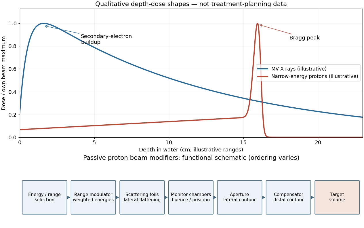
A passively scattered proton therapy beam uses distinct devices to control lateral spread, range and distal shape. The lower panel of the figure gives a functional schematic; the exact ordering varies among beamlines. An energy selector or range shifter sets the maximum range. A stepped range-modulation wheel or ridge filter gives a weighted collection of proton energies, forming the spread-out Bragg peak. One or more scattering foils broaden the narrow beam; a double-scattering system can improve lateral uniformity. Ionization chambers monitor delivered fluence and position. A patient-specific aperture or collimator blocks unwanted lateral regions. A shaped range compensator makes the remaining range vary across the field, matching the distal target boundary. Their effects must be combined: lateral collimation alone cannot flatten the depth distribution, and an energy modulator alone cannot set the lateral contour.^[ref]

For a megavoltage X-ray beam, the surface absorbed dose is below the subsurface maximum. Photons generate energetic secondary electrons, mainly through Compton scattering; the downstream electron fluence initially builds up until approximate charged-particle equilibrium is established. Beyond this buildup region, decreasing primary photon fluence, scattering and geometric spreading make the depth-dose curve fall gradually. A penetrating photon beam has a substantial exit dose.

A nearly monoenergetic proton beam deposits a moderate entrance dose, then a sharp Bragg peak near the end of its range. As nonrelativistic protons slow, their electronic stopping power rises approximately as $1/v^2$ over the relevant part of the track. Once the protons stop, the dose falls steeply. Range straggling and energy spread broaden the peak; nuclear interactions add a smaller nonideal tail, so an exact hard cutoff is an idealization. Superposing appropriate incident energies produces a spread-out Bragg peak covering an extended target.^[ref]

The label MV for an X-ray treatment beam specifies the nominal accelerating potential of the electron accelerator. Its bremsstrahlung beam is a broad photon energy spectrum with an endpoint of order $eV$, not a monoenergetic beam whose individual photons all carry the quoted numerical energy. Proton therapy beam energies can instead be specified directly in MeV per incident proton.

In the ideal unscattered coincidence model, let a positron annihilation occur at position $s$ on a coincidence line of response connecting detectors $A$ and $B$. Its two oppositely directed photons must both survive. Their independent attenuation factors multiply:The source position cancels because the complementary path integrals span the whole chord. In a uniform slab of chord length $L$, the same argument is $e^{-\mu s}{e}^{-\mu (L-s)}=e^{-\mu L}$. Therefore attenuation correction requires the full linear attenuation coefficient map along the chord, but not the depth of the particular annihilation along that chord. This argument addresses attenuation of true PET coincidences; scatter, random coincidences and detector efficiency need their own corrections.

A CT number is a dimensionless relative attenuation measure, conventionally $H=1000({\mu }_{\mathrm{CT}}-{\mu }_{\mathrm{water},\mathrm{CT}})/{\mu }_{\mathrm{water},\mathrm{CT}}$. The X-ray spectrum used in computed tomography has an effective energy far below $511\mathrm{keV}$ and is polychromatic. Its photoelectric absorption contribution depends strongly on composition, whereas water and soft-tissue attenuation at the positron emission tomography energy is mainly Compton scattering. Thus a CT number is neither a $511\mathrm{keV}$ linear attenuation coefficient nor an energy-independent mass attenuation coefficient.

The usual conversion calibrates a piecewise linear or bilinear relation between CT numbers and $\mu (511\mathrm{keV})$. The air–water branch models predominantly density differences in lung and soft tissue; a separate water–bone branch accounts for the different energy dependence of mineralized tissue. The calibration depends on the computed tomography spectrum. After geometric registration, the resulting linear attenuation coefficient map is forward projected along each coincidence line of response to obtain $\exp (\int {\mu }_{511}ds)$. If a mass coefficient is stored, its conversion to a linear coefficient must also include mass density. Unusual high-atomic-number materials can violate the simple tissue calibration, so the conversion is a physical material model, not a universal arithmetic rescaling.^[ref][ref]

For photons, the total mass attenuation coefficient sums contributions from photoelectric absorption, Compton scattering, coherent Rayleigh scattering, and pair production in nuclear or electronic fields when above their thresholds. At sufficiently high photon energies, photonuclear reactions can also contribute. Attenuation counts removal from the incident narrow beam, including scattering without complete local deposition of the original energy.

In water at both specified energies, Compton scattering dominates. At $140\mathrm{keV}$, photoelectric absorption and coherent Rayleigh scattering make smaller contributions; at $511\mathrm{keV}$ these are still less important. Nuclear-field pair production is impossible below $2m_e{c}^2=1.022\mathrm{MeV}$, so it occurs in neither example. The positrons used to produce the fluorine-18 annihilation radiation do not change that threshold for interactions of its $511\mathrm{keV}$ photons in water.

Strictly, $\mu$ is a linear attenuation coefficient, whereas $\mu /\rho$ is a mass attenuation coefficient; the source's wording blurs these units. The mass energy-absorption coefficient ${\mu }_{\mathrm{en}}/\rho$ weights the fraction of incident photon energy transferred to charged particles and retained after radiative losses, rather than simply counting all removals. Coherent scattering contributes attenuation with negligible energy transfer. A photon deflected by Compton scattering can carry much of the original energy away. One often writes ${\mu }_{\mathrm{en}}=(1-g){\mu }_{\mathrm{tr}}$, with $g$ the fraction of secondary charged-particle kinetic energy lost radiatively. Under charged-particle equilibrium, multiplying photon energy fluence by ${\mu }_{\mathrm{en}}/\rho$ gives the absorbed dose; that equilibrium condition matters near interfaces and in buildup regions.^[ref]

For a narrow, well-collimated photon beam, scattered photons are rejected and the uncollided intensity obeys the Beer-Lambert law, $I(x)=I(0)e^{-\mu x}$. With water mass density $\rho \simeq 1\mathrm{g}\mathrm{c}{\mathrm{m}}^{-3}$, the linear attenuation coefficient is $\mu =\rho (\mu /\rho )$. The half-value layer is thereforeThus the annihilation photons associated with the fluorine-18 source require about $1.60$ times as much water for the same attenuation as the technetium-99m photons. The $511\mathrm{keV}$ here is the annihilation photon energy, not the variable kinetic energy of an emitted Positron. A broad-beam measurement admitting scattered photons would require a buildup correction and would not have this simple transmission interpretation.^[ref]

Let $I$ denote the requested integral. Symmetry and the period of ${\sin }^2\theta$ make the corresponding integral over $0\le \theta \le 2\pi$ equal to $4I$. With $z=e^{i\theta }$, this becomesThe denominator factors as $-2(z^2-1/2)(z^2-2)$. The two poles inside the unit circle are $z=\pm 1/\sqrt{2}$. Each residue is $1/(6i)$, because the derivative of the polynomial denominator there is $6z$. The residue theorem gives $4I=2\pi /3$, so

For $t>0$, close the real-axis contour in the upper half-plane: $|e^{izt}|=e^{-t\mathrm{Im}z}$ supplies decay. The only enclosed simple pole is $z=i$, with residue $e^{-t}/(2i)$. Thus $h(t)=2\pi i{e}^{-t}/(2i)=\pi e^{-t}$.

For $t<0$, close downwards. The clockwise orientation contributes $-2\pi i$ times the residue $e^t/(-2i)$ at $z=-i$, givingAt $t=0$, direct integration of $1/(1+p^2)$ gives $\pi$, consistent with the continuous extension. The large arc tends to zero by Jordan's lemma for nonzero $t$, or the denominator estimate when $t=0$.

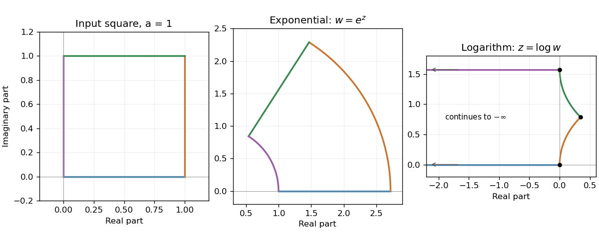
Use the complex logarithm with $0\le \arg w\le \pi /2$ on the nonzero points of the first-quadrant square. Put $z=x+iy=\log |w|+i\arg w$. The square bounds $\mathrm{Re}w,\mathrm{Im}w\le a$ giveThe two edges meeting at $w=0$ map to the horizontal half-lines $y=0$ and $y=\pi /2$, extending indefinitely to the left. The other edges map to $x=\log a-\log \cos y$ for $0\le y\le \pi /4$ and $x=\log a-\log \sin y$ for $\pi /4\le y\le \pi /2$. They meet at $\log (a\sqrt{2})+i\pi /4$.

The angles are preserved at $a$, $a(1+i)$ and $ia$. There $d\log w/dw=1/w$ is finite and nonzero. The origin is a branch point, has no finite logarithmic image, and supplies no fourth finite vertex at which angle preservation could be asserted.

Writing $z=x+iy$ gives $|w|=e^x$ and $\arg w=y$. Thus the closed square maps to the annular sectorIts horizontal edges become radial segments and its vertical edges become circular arcs. Each radial tangent is perpendicular to the tangent of its adjoining circle, so the four interior angles remain $\pi /2$. Equivalently, the complex derivative $e^z$ is nonzero at every vertex and the map is conformal there.

No region maps onto the entire finite complex plane: $e^z$ is never zero. Its image on $\mathbb{C}$ is $\mathbb{C}\setminus \{0\}$. A fundamental strip such asmaps bijectively onto that punctured plane, because $e^{x+iy}=e^x{e}^{iy}$. The half-open strip supplies one representative of each angle; it is not an open domain. An open strip of height $2\pi$ omits a ray as well. The missing zero is approached only in the limit $x\to -\infty$.

A conformal map preserves the magnitude and orientation of angles between intersecting smooth curves locally. For a complex holomorphic function, the condition at $z_0$ is $f^{\prime }(z_0)\ne 0$: the first-order change $\delta w=f^{\prime }(z_0)\delta z$ rotates and uniformly scales every tangent vector by the same complex factor. This local statement does not require a globally one-to-one map.

Take $g(z)=L(z{)}^3/z^3$ on the same logarithm branch. At zero, $L(z{)}^3=-z^3+O(z^4)$, so the apparent singularity is removable and the closed contour integral is zero. The bank difference isThe circular contributions vanish by the previous estimates with the third power of the logarithm. ConsequentlyThe last integral is $1/2$, givingIncreasing the logarithm power has converted the desired real integral into a jump across a branch cut, while removing the pole inside the contour.

Use the positive orientation shown in the source: the upper bank runs outwards and the lower bank returns towards one. On those banks the logarithm branch has values $\ell -i\pi$ and $\ell +i\pi$, respectively, with $\ell =\log (x-1)$. Their squared difference is $-4i\pi \ell$. The residue theorem therefore givesand henceThe large-circle contribution is $O(R^{-2}{\log }^{2}R)$ and the small circle about one contributes $O(\epsilon |\log \epsilon {|}^2)$, both tending to zero. These estimates justify replacing the closed contour integral by its two cut-bank integrals.

Choose the principal logarithm, so $L(z)=\mathrm{Log}(1-z)$ has branch cut $[1,\infty )$. Near zero its Taylor series givesThus zero is a simple pole of residue one, and one is a logarithmic branch point. The function is holomorphic on $\mathbb{C}\setminus (\{0\}\cup [1,\infty ))$ with this branch. Infinity is also a branch point in the extended-plane description; the function's decay there along the cut plane does not make it a single-valued holomorphic function through infinity.

The one-step expected price multiplier under the stated physical probability is $1.1p+0.9(1-p)=0.9+0.2p$. Independence lets the expectation of the product factorize, givingThe same expression follows by summing the four binomial endpoint probabilities times their prices. This is a physical-measure expectation; option replication below uses a separately determined risk-neutral probability.