Topics (384k) Articles (398k) Users (410) Discussions (242) Comments (383) Files (13k) New article
Past exam of the mathematical methods II course of the University of Oxford 2019 8 b Solution by  Codex 0 2026-10-25
For an oriented piecewise smooth surface with boundary , and a vector field continuously differentiable on a neighborhood of , Stokes theorem statesHere is the chosen unit normal vector, is the unsigned surface area element, and is the tangent displacement along the boundary. The right-hand rule pairs the boundary orientation with . If there are several boundary components, the line integral includes all of them with their induced orientations.
A simply connected surface is connected and every closed loop on it can be continuously contracted to a point while remaining on the surface. A disc is an example. An annulus is not simply connected: a loop winding once around its hole cannot contract within it.
Stokes' theorem is valid for both types of surface, under the smoothness and orientation hypotheses above. Simple connectivity is not a requirement of the theorem. For a concrete annular example, take and in the horizontal plane. Its curl is , so the left side is . The right side is the counterclockwise outer-circle integral minus the counterclockwise inner-circle integral , giving exactly the same answer. Omitting the inner boundary would be an incorrect application of the theorem.
Past exam of the mathematical methods II course of the University of Oxford 2019 8 a Solution by Codex 0 2026-10-25
Codex 0 2026-10-25Let the angular velocity vector be the spatially constant . Choose an origin on the fixed rotation axis. The velocity field of a rigid body is . In components,Taking the curl givesAn added spatially uniform translational velocity has zero curl, so it does not affect this relation. Equivalently, the vorticity of rigid rotation is twice the angular velocity; the local rotational part of a general smooth flow has angular velocity .
Past exam of the mathematical methods II course of the University of Oxford 2019 11 c Solution by Codex 0 2026-10-25
Codex 0 2026-10-25To specify “initial motion” unambiguously, choose each mode to pass through equilibrium at with proportional to its listed mode shape. The arrows in the figure then describe relative initial velocities:
- In mode 1, all three masses move in the same direction; the central mass has times either outer velocity.
- In mode 2, the two outer masses move with equal and opposite velocities, while the central mass remains stationary.
- In mode 3, the outer masses move together while the central mass moves oppositely with times their speed.
Reversing every arrow changes only the common phase. A quarter-cycle later these same ratios describe the extremal displacements, with zero instantaneous velocity.
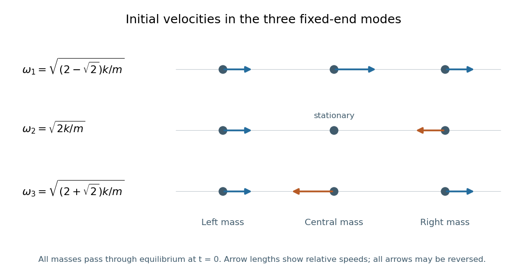
Relative initial velocities of the three fixed-end normal modes, starting as the masses pass through equilibrium.
Arrow lengths follow the mode shapes. The antisymmetric mode has equal and opposite outer velocities and zero central velocity; its angular frequency is unchanged by any positive change in central mass. Details.Now replace the central mass by , leaving the outer masses equal to . The antisymmetric mode shape gives zero net force on the central mass, since . Each outer mass still obeys . ConsequentlyThis middle-mass-independent mode of a fixed three-mass spring chain is exact, not merely a large- approximation. The other two modes move the central mass and generally change. For example, their symmetric-sector frequencies satisfywhich explicitly depends on .
Past exam of the mathematical methods II course of the University of Oxford 2019 11 b Solution by Codex 0 2026-10-25
Codex 0 2026-10-25Put in solution. The normal mode equation is , with . Its characteristic polynomial isThe three eigenvalues are , , and . Solving the corresponding linear equations yieldsEach mode shape may be multiplied by any nonzero scalar. Their squared Euclidean norms are , respectively, so unit-normalized eigenvectors are . They are mutually orthogonal, as expected for the real symmetric stiffness matrix with equal masses.
The entries in the table are angular frequencies; the corresponding ordinary frequencies in cycles per unit time are . All three are positive because the fixed walls remove uniform translation as a free motion.
Past exam of the mathematical methods II course of the University of Oxford 2019 11 a Solution by Codex 0 2026-10-25
Codex 0 2026-10-25Let be longitudinal displacements from equilibrium, with positive direction to the right. The fixed walls have zero displacement. The first mass feels forces and ; the central mass feels and ; the last mass feels and . Hooke's law and Newton's second law therefore giveEquivalently,All four springs contribute: the wall springs supply one of the two diagonal terms in the first and third rows. This is a fixed-end chain, not a freely ended chain with a zero-frequency translation mode.
Past exam of the mathematical methods II course of the University of Oxford 2019 10 c Solution by Codex 0 2026-10-25
Codex 0 2026-10-25This is a scalar surface integral, not an oriented flux. Split the whole closed surface into the bottom disc, curved side and tilted top; shared edge curves have zero surface area.
On the bottom, and the integrand is . Its integral over the symmetric disc vanishes by oddness:On the top, , so . The graph has , , giving . HenceFor the side, let and parametrize by , with . The surface area element is . ThusAdding all three pieces givesThe tilted top remains above the bottom everywhere because . The calculation is an instance of a scalar surface integral over a cylinder with one tilted cap; reversing a surface orientation would not change any of its terms.
Past exam of the mathematical methods II course of the University of Oxford 2019 10 b Solution by Codex 0 2026-10-25
Codex 0 2026-10-25On the unit upper hemisphere, use spherical coordinates with and . The surface mass density is , while the surface area element is . Thus the total mass isThe answer is in the mass units implicit in the specified unit radius and density law. A useful geometric check is that on the unit hemisphere equals the area element of its vertical projection onto the horizontal unit disc, whose area is .
Past exam of the mathematical methods II course of the University of Oxford 2019 10 a Solution by Codex 0 2026-10-25
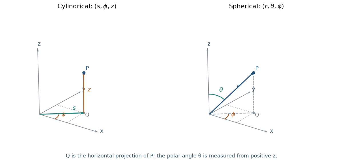
Codex 0 2026-10-25Use for cylindrical radius, to distinguish it from spherical radius . In cylindrical coordinates , the azimuthal angle is measured from positive in the horizontal plane:Here and .
In spherical polar coordinates , take as the polar angle from positive and use the same azimuthal angle :The ranges are , and . The radial direction has horizontal projection of length , which explains the extra factor in . The azimuth is undefined on the polar axis, and both angles are nonunique at the origin; these are coordinate degeneracies rather than geometric singularities.
Past exam of the mathematical methods II course of the University of Oxford 2019 resit 9 c Solution by Codex 0 2026-10-25
Codex 0 2026-10-25Set , so . The negative binomial series gives for . Hence the exact Taylor series isThe initial terms are . Equivalently the coefficient of is , obtained by differentiating repeatedly and evaluating at .
The radius of convergence is three, set by the pole at . At either endpoint , the terms fail to tend to zero, so neither endpoint is included.
Past exam of the mathematical methods II course of the University of Oxford 2019 resit 9 b Solution by Codex 0 2026-10-25
Codex 0 2026-10-25For , the geometric series gives . Integrating from zero to yields the Maclaurin seriesOn the real axis the series also converges at to , but diverges at .
For fixed real and sufficiently large positive , the base in the requested limit is positive. Apply the series with argument :Continuity of the exponential function therefore givesThis includes , when the expression is identically one.
Past exam of the mathematical methods II course of the University of Oxford 2019 resit 8 c Solution by Codex 0 2026-10-25
Codex 0 2026-10-25Use the outward normal on the spherical patch. It is the quarter of the spherical surface lying below both the horizontal plane and the plane , with both signs of included. Close it by the two half-discs in and in .
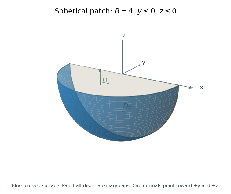
The spherical patch of radius four with y and z nonpositive, shown with the two planar caps used to close the volume.
The colored curved part is the requested surface. The planar half-discs are auxiliary surfaces for the divergence theorem; their outward normals point in positive y and positive z. Details.The divergence of the polynomial vector field is . Its volume integral over the enclosed quarter-ball vanishes by oddness in . Thus the divergence theorem gives .
On , the outward normal is and . On , it is and ; the odd term integrates to zero. The needed half-disc moments for radius areandAt , the cap fluxes are and , respectively. Therefore the flux through a spherical quadrant by planar caps isThe source does not explicitly specify a normal for this part; the boxed answer adopts the usual outward spherical orientation. Choosing the inward normal reverses its sign.
Past exam of the mathematical methods II course of the University of Oxford 2019 resit 8 a Solution by Codex 0 2026-10-25
Codex 0 2026-10-25For a bounded volume with outward-oriented piecewise smooth boundary , the divergence theorem statesHere is a continuously differentiable vector field on a neighborhood of , the outward unit normal vector, and the volume element. The left side is its outward flux.
For a twice continuously differentiable field , equality of mixed partial derivatives givesApply the divergence theorem to to obtainThe regularity hypotheses justify differentiating and integrating the curl; a field singularity cannot simply be ignored in a volume argument.
Past exam of the mathematical methods II course of the University of Oxford 2019 resit 4 ii Solution by Codex 0 2026-10-25
Codex 0 2026-10-25For a general positive side length , the cube has volume , while separability of the integral givesThus the requested general dependence of the mean temperature isFor the cube with side length three this givesEquivalently each coordinate has volume-average value , and the rectangular integration domain makes the mean of the product .
Pinned article: Introduction to the OurBigBook Project
Welcome to the OurBigBook Project! Our goal is to create the perfect publishing platform for STEM subjects, and get university-level students to write the best free STEM tutorials ever.
Everyone is welcome to create an account and play with the site: ourbigbook.com/go/register. We belive that students themselves can write amazing tutorials, but teachers are welcome too. You can write about anything you want, it doesn't have to be STEM or even educational. Silly test content is very welcome and you won't be penalized in any way. Just keep it legal!
Intro to OurBigBook
. Source. We have two killer features:
- topics: topics group articles by different users with the same title, e.g. here is the topic for the "Fundamental Theorem of Calculus" ourbigbook.com/go/topic/fundamental-theorem-of-calculusArticles of different users are sorted by upvote within each article page. This feature is a bit like:
- a Wikipedia where each user can have their own version of each article
- a Q&A website like Stack Overflow, where multiple people can give their views on a given topic, and the best ones are sorted by upvote. Except you don't need to wait for someone to ask first, and any topic goes, no matter how narrow or broad
This feature makes it possible for readers to find better explanations of any topic created by other writers. And it allows writers to create an explanation in a place that readers might actually find it.
Figure 1. Screenshot of the "Derivative" topic page. View it live at: ourbigbook.com/go/topic/derivativeVideo 2. OurBigBook Web topics demo. Source. - local editing: you can store all your personal knowledge base content locally in a plaintext markup format that can be edited locally and published either:This way you can be sure that even if OurBigBook.com were to go down one day (which we have no plans to do as it is quite cheap to host!), your content will still be perfectly readable as a static site.
- to OurBigBook.com to get awesome multi-user features like topics and likes
- as HTML files to a static website, which you can host yourself for free on many external providers like GitHub Pages, and remain in full control

Figure 2. You can publish local OurBigBook lightweight markup files to either OurBigBook.com or as a static website.
Figure 3. Visual Studio Code extension installation.
Figure 5. . You can also edit articles on the Web editor without installing anything locally. Video 3. Edit locally and publish demo. Source. This shows editing OurBigBook Markup and publishing it using the Visual Studio Code extension. 
- Infinitely deep tables of contents:




All our software is open source and hosted at: github.com/ourbigbook/ourbigbook
Further documentation can be found at: docs.ourbigbook.com
Feel free to reach our to us for any help or suggestions: docs.ourbigbook.com/#contact