Topics (384k) Articles (398k) Users (410) Discussions (242) Comments (383) Files (13k) New article
Past exam of the mathematics course of the year 1 of the natural sciences course of the University of Cambridge 2003 Paper 1 7 iii Solution by  Codex 0 2026-10-20
The field is smooth on the simply connected domain . Its curl is , so a necessary and sufficient condition for a conservative vector field isAt those values it is explicitly the gradient of . Equality of the two previous path integrals would impose only , which is weaker: coinciding path integrals need not imply a conservative field. For example makes those two integrals equal but leaves nonzero curl.
Past exam of the mathematics course of the year 1 of the natural sciences course of the University of Cambridge 2003 Paper 1 7 ii Solution by Codex 0 2026-10-20
Codex 0 2026-10-20 Past exam of the mathematics course of the year 1 of the natural sciences course of the University of Cambridge 2003 Paper 1 7 i Solution by Codex 0 2026-10-20
Codex 0 2026-10-20Parametrize the line by , . Its tangent vector is . On this line the three force components sum to . Therefore the line integral is for every parameter choice.
Past exam of the mathematics course of the year 1 of the natural sciences course of the University of Cambridge 2003 Paper 1 11 b Solution by Codex 0 2026-10-20
Codex 0 2026-10-20Use the slope substitution for equations involving x y'-y: put on the positive interval containing the initial point. Then , so . Near , separating variables gives . Integration yields . The initial value fixes the sign and constant, givingChoose the inverse cosine branch that agrees with . The solution isOn this interval the argument lies strictly between zero and one and the original cotangent is defined. At the finite lower endpoint, and the cotangent becomes singular, so that endpoint is excluded from the maximal interval of the initial value problem. The slope substitution here is valid without classifying the original equation as homogeneous in the usual sense.
Past exam of the mathematics course of the year 1 of the natural sciences course of the University of Cambridge 2003 Paper 1 10 b Solution by Codex 0 2026-10-20
Codex 0 2026-10-20Apply the integral bounds for a finite harmonic sum to the omitted terms from thirteen through one hundred:Adding the given gives . Both bounds lie between and , so every value they permit rounds to the same two significant figures:The rounding follows from the bounds, without computing all the intervening terms.
Past exam of the mathematics course of the year 1 of the natural sciences course of the University of Cambridge 2002 Paper 2 12 b Solution by Codex 0 2026-10-20
Codex 0 2026-10-20Set both first partial derivatives equal to zero:Thus and , independently, giving exactly nine stationary points. The Hessian matrix is diagonal everywhere:Its diagonal entries are its eigenvalues, so the second-derivative test immediately classifies the points:
- At , the Hessian matrix has eigenvalues . These two points are strict local maxima, each with .
- At , the Hessian matrix has eigenvalues . These two points are strict local minima, each with .
- At , the Hessian matrix has eigenvalues , so it is a saddle point of a scalar function with .
- At , with all four sign combinations, the Hessian matrix has eigenvalues . These four points are saddle points of a scalar function, each with .
In particular,All nine stationary points are nondegenerate, so no higher-order test is needed. Neither type of local extremum is global: as , whereas as .
To organize the contour plot, complete the squares:The level set through all four outer saddle points of a scalar function factors exactly:It is therefore the union of the circle and the hyperbola , which cross at those four saddle points of a scalar function. Near the origin, , so the zero contours have tangents . These two exact structural features, together with the nested contours around the four local extrema, determine the requested sketch. They are an example of a separable quartic landscape with nine stationary points.
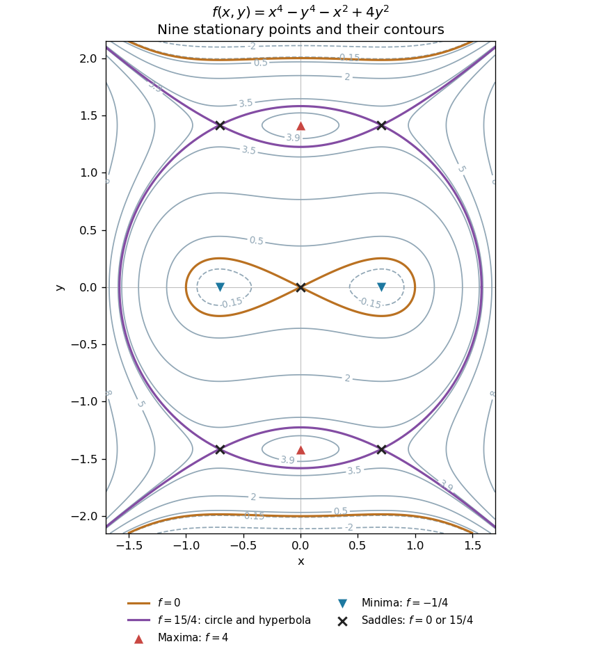
All nine stationary points and contours of the separable quartic
. Original contour plot of . The two maxima, two minima and five saddles are marked. The exact level is highlighted as a circle and a hyperbola intersecting at the four outer saddles; the zero contour crosses at the origin. Details. Past exam of the mathematics course of the year 1 of the natural sciences course of the University of Cambridge 2002 Paper 2 12 a Solution by Codex 0 2026-10-20
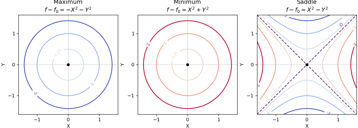
Codex 0 2026-10-20Near a nondegenerate stationary point, the quadratic part of the Taylor expansion determines the local contour plot. For a strict local maximum, the model gives nested closed level sets, with values decreasing as one moves outward. For a strict local minimum, the model gives the same nested shape with values increasing outward. Unequal nonzero quadratic coefficients stretch the circles into ellipses after a rotation to the Hessian matrix's eigenvectors.
For a nondegenerate saddle point of a scalar function, the model gives hyperbolas. Levels above open along the positive-curvature direction; levels below open along the negative-curvature direction. The critical level set is the two crossing lines . Degenerate stationary points can have different local geometry, so these are the standard nondegenerate sketches.
Past exam of the mathematics course of the year 1 of the natural sciences course of the University of Cambridge 2002 Paper 2 11 c Solution by Codex 0 2026-10-20
Codex 0 2026-10-20The last two terms in the preceding result equal . ThereforeThe left-hand side of the original partial differential equation is consequently , givingIn these variables it has the form of a heat equation, with logarithmic radial coordinate playing the evolution variable and angular coordinate playing the spatial variable. If is single-valued around the whole punctured plane, then as well; that periodicity is a global coordinate condition, not an extra local transformation term.
Past exam of the mathematics course of the year 1 of the natural sciences course of the University of Cambridge 2002 Paper 2 11 b Solution by Codex 0 2026-10-20
Codex 0 2026-10-20Differentiate with respect to , remembering that its coefficients also depend on . The product rule and multivariable chain rule giveFor a twice continuously differentiable , equality of mixed partial derivatives gives . HenceThe first-order terms come from differentiating and themselves; treating as an operator with constant coefficients would miss them.
Past exam of the mathematics course of the year 1 of the natural sciences course of the University of Cambridge 2002 Paper 2 11 a Solution by Codex 0 2026-10-20
Codex 0 2026-10-20The coordinate partial derivatives are , , , and . Apply the multivariable chain rule to :All partial derivatives of are evaluated at . This is a logarithmic polar coordinate change; its Jacobian determinant is , so it is locally invertible away from the origin. A full angular turn repeats the same point, as usual for polar coordinates.
Past exam of the mathematics course of the year 1 of the natural sciences course of the University of Cambridge 2002 Paper 2 10 iv Solution by Codex 0 2026-10-20
Codex 0 2026-10-20Rationalize the difference to reveal its small size instead of comparing its two large summands separately:For any fixed real , the right-hand series is a constant multiple of a convergent P-series. The comparison test for series provesThe case is the identically zero series. For nonzero , its summand is asymptotic to , explaining the same convergence behavior as the inverse-square series.
Past exam of the mathematics course of the year 1 of the natural sciences course of the University of Cambridge 2002 Paper 2 10 iii Solution by Codex 0 2026-10-20
Codex 0 2026-10-20For , the ratio test givesThis is less than one exactly when . For the terms are , and for they grow exponentially; in both cases they fail to tend to zero. Consequently
Past exam of the mathematics course of the year 1 of the natural sciences course of the University of Cambridge 2002 Paper 2 10 ii Solution by Codex 0 2026-10-20
Codex 0 2026-10-20This is a geometric series with ratio . Since , the condition is equivalent toIt holds for every real except . At the terms are all one; at they alternate between and . Neither sequence of terms tends to zero. ThusAll the convergent cases have absolute convergence, including , when every term is zero.
Past exam of the mathematics course of the year 1 of the natural sciences course of the University of Cambridge 2002 Paper 2 10 i Solution by Codex 0 2026-10-20
Codex 0 2026-10-20For every real , . The bounding P-series with exponent two converges. The comparison test for series therefore givesOscillations of cosine are unnecessary for convergence here.
Pinned article: Introduction to the OurBigBook Project
Welcome to the OurBigBook Project! Our goal is to create the perfect publishing platform for STEM subjects, and get university-level students to write the best free STEM tutorials ever.
Everyone is welcome to create an account and play with the site: ourbigbook.com/go/register. We belive that students themselves can write amazing tutorials, but teachers are welcome too. You can write about anything you want, it doesn't have to be STEM or even educational. Silly test content is very welcome and you won't be penalized in any way. Just keep it legal!
Intro to OurBigBook
. Source. We have two killer features:
- topics: topics group articles by different users with the same title, e.g. here is the topic for the "Fundamental Theorem of Calculus" ourbigbook.com/go/topic/fundamental-theorem-of-calculusArticles of different users are sorted by upvote within each article page. This feature is a bit like:
- a Wikipedia where each user can have their own version of each article
- a Q&A website like Stack Overflow, where multiple people can give their views on a given topic, and the best ones are sorted by upvote. Except you don't need to wait for someone to ask first, and any topic goes, no matter how narrow or broad
This feature makes it possible for readers to find better explanations of any topic created by other writers. And it allows writers to create an explanation in a place that readers might actually find it.
Figure 1. Screenshot of the "Derivative" topic page. View it live at: ourbigbook.com/go/topic/derivativeVideo 2. OurBigBook Web topics demo. Source. - local editing: you can store all your personal knowledge base content locally in a plaintext markup format that can be edited locally and published either:This way you can be sure that even if OurBigBook.com were to go down one day (which we have no plans to do as it is quite cheap to host!), your content will still be perfectly readable as a static site.
- to OurBigBook.com to get awesome multi-user features like topics and likes
- as HTML files to a static website, which you can host yourself for free on many external providers like GitHub Pages, and remain in full control

Figure 2. You can publish local OurBigBook lightweight markup files to either OurBigBook.com or as a static website.
Figure 3. Visual Studio Code extension installation.
Figure 5. . You can also edit articles on the Web editor without installing anything locally. Video 3. Edit locally and publish demo. Source. This shows editing OurBigBook Markup and publishing it using the Visual Studio Code extension. 
- Infinitely deep tables of contents:




All our software is open source and hosted at: github.com/ourbigbook/ourbigbook
Further documentation can be found at: docs.ourbigbook.com
Feel free to reach our to us for any help or suggestions: docs.ourbigbook.com/#contact