Core accretion builds a solid core and then a massive gaseous envelope before protoplanetary disk dispersal. The solid and gas stages overlap; this is not direct collapse of a whole disk patch.

In a protoplanetary disk, refractory grains and, beyond a snow line, condensed ices provide solids. Settling and protoplanetary dust coagulation build aggregates, but fragmentation, bouncing and radial drift of solids in a gas disk can interrupt simple sticking. Concentration processes such as the streaming instability can produce dense particle structures that collapse into planetesimals. Subsequent collisions build planetary embryos; alternatively, embryos can efficiently capture drifting particles through gas-assisted pebble accretion. Neither the initial planetesimal population nor unrestricted growth through every size should be assumed without a mechanism.

For gravitationally focused growth of a planetary core, the two-body capture cross-section isAn illustrative thin-disk estimate is ${\dot{M}}_c\sim {\Sigma }_s\Omega {\sigma }_{\mathrm{coll}}$, up to geometry and velocity-distribution factors. At fixed solid density and random speed, strong gravitational focusing gives ${\dot{M}}_c\propto M_c^{4/3}$: runaway planetesimal growth. As large embryos stir the smaller bodies, encounter speeds increase and focusing weakens, giving oligarchic growth. Consuming the local feeding zone leads toward an isolation mass; radial supply, migration and mergers can extend growth. Snow lines can increase the solid reservoir, but a distant core also grows more slowly because orbital times are longer.^[ref]

A growing core binds gas over a scale limited by the smaller of its Bondi radius and Hill radius. The envelope approximately satisfiesAn equation of state, disk boundary conditions, and radiative or convective energy transport close the structure. In an optically thick radiative region,Here $\kappa$ is opacity; an unstable radiative gradient instead drives convection. Solid accretion releases roughly $L_s\sim G{M}_c{\dot{M}}_c/R_c$, heating and supporting the envelope. Gas capture consequently depends on cooling, not just whether the potential can bind gas instantaneously.

The envelope loses energy on a Kelvin-Helmholtz cooling time, $t_{\mathrm{KH}}\sim |E_{\mathrm{env}}|/L$. Lower grain opacity, higher core mass, or reduced solid-accretion heating can accelerate contraction. The critical core mass for gas accretion is therefore model dependent; “of order ten Earth masses” is a common scale, not a universal switch. As envelope self-gravity becomes important and the gas and solid masses become comparable, contraction permits still more gas capture, producing runaway gas accretion. The classical sequence has a rapid solid-growth phase, a slower envelope-growth phase, and accelerated gas accumulation.^[ref]

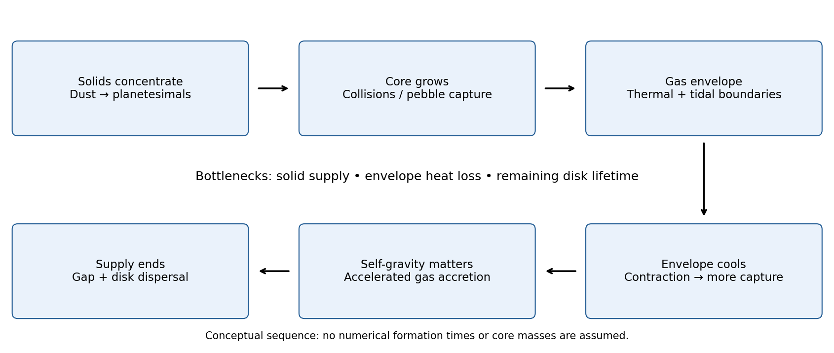
The decisive race is $t_{\mathrm{core}}+t_{\mathrm{envelope}}\lesssim t_{\mathrm{disk}}$. Failure to cool or obtain a sufficiently large core before gas removal leaves a smaller solid or ice-rich planet. Successful growth is ultimately limited by disk supply, gap opening by a planet, and dispersal; a gap does not completely seal off accretion. Angular-momentum exchange drives planetary migration, so the observed orbit need not be the formation radius. Accretion-shock radiation and subsequent contraction set the young giant's entropy and luminosity; final core mass, envelope enrichment and orbital location depend on the whole growth history, not on one fixed threshold. The necessary cooling, supply and orbital constraints make the model testable rather than an assertion that every embryo must become a gas giant.

A stable sinusoidal radial-velocity semi-amplitude can be stellar reflex motion caused by a companion on a nearly circular orbit. The amplitude is compatible with a giant planet; a low-mass star or brown dwarf viewed nearly face-on can mimic the same projected motion, but requires an increasingly unlikely orientation. Starspots and magnetically suppressed convection can produce a rotational stellar activity signal on a ten-day timescale; contemporaneous photometry, activity indicators and stellar spectral-line bisector and other profile changes distinguish these from a clean common Doppler shift. Solar-like stellar oscillations ordinarily have much shorter periods, so a coherent ten-day oscillation of an otherwise ordinary solar-type dwarf is less plausible. Instrumental drift, sampling aliases and blended spectra also need checking. A sinusoid alone does not establish a planetary origin, and the data do not assign numerical probabilities to these alternatives.

For the minimum companion mass from radial velocity, take a circular two-body orbit and initially $M_{\star }=M_{\odot }$. The exact relation and its low-mass limit areWith $\sin i=1$,Here $a=[G{M}_{\star }{P}^2/(4{\pi }^2){]}^{1/3}$ is the relative orbital semi-major axis. Nonzero orbital eccentricity multiplies the inferred $M_p\sin i$ by $\sqrt{1-e^2}$ at fixed measured $K,P$, but the sinusoidal model motivates $e=0$ here.

For the radial-velocity sensitivity limit at fixed planet mass, use $K=M_p\sin i\sqrt{G/(M_{\star }a)}$ and interpret the stated detection scale as a semi-amplitude threshold $K_{\min }$. The largest distance occurs for $\sin i=1$:For an inclination $i$, this boundary is smaller by ${\sin }^{2}i$. The result assumes adequate time coverage and neglects the stipulated stellar noise. If the detection scale instead denotes a full peak-to-peak excursion, set $K_{\min }$ to half that scale; $a_{\max }$ then increases fourfold.

The stellar-mass scaling of radial-velocity planet estimates changes these inferences because Kepler's third law and the stellar reflex response depend on the stellar mass. At fixed $K,P$, $M_p\sin i\propto M_{\star }^{2/3}$ and $a\propto M_{\star }^{1/3}$, whereas the fixed-mass detectability boundary scales as $M_{\star }^{-1}$. ThereforeThe observed period and amplitude are unchanged. The stellar radius does not enter these leading dynamical estimates, but is crucial for the exoplanet transit inference.

For the transiting companion, assume an opaque spherical planet, negligible transit dilution and negligible limb darkening. Its radius ratio is $k=R_p/R_{\star }=\sqrt{\delta }=0.03873$, henceUsing the revised stellar mass and a circular orbit gives $a=0.01850\mathrm{au}$ and $A=a/R_{\star }=7.957$. Interpret the duration as the total first-to-fourth-contact duration $T_{14}$. The impact parameter from total transit duration follows from the total duration of a circular planetary transit:This is noncentral but not grazing: $b<1-k$. The small-planet straight-chord approximation gives $b\simeq 0.845$; retaining finite $R_p$ and orbital curvature gives the stated value. A duration measured between other contacts needs the corresponding contact formula. Unknown orbital eccentricity and argument of periapsis change the transverse speed and prevent a unique unconstrained $b$; the numerical estimate is conditional on the stated circular model.^[ref]

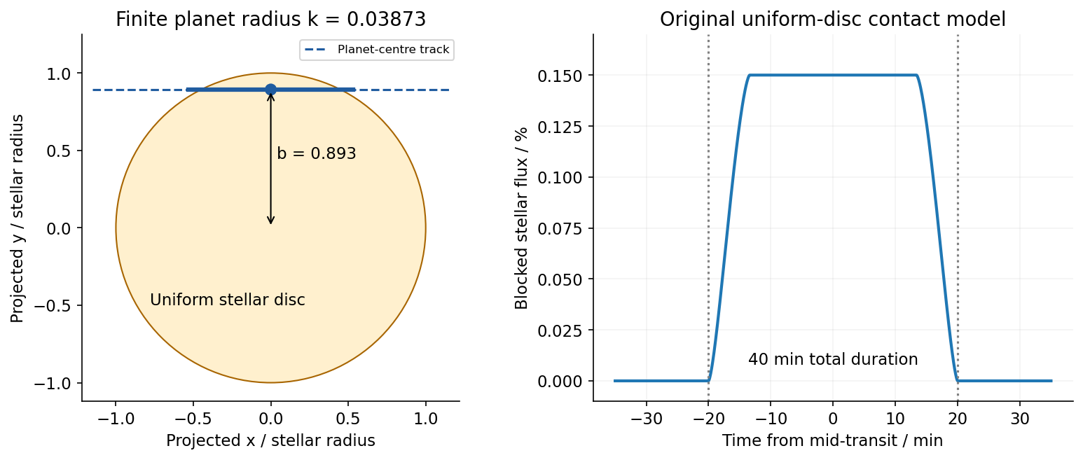
Because the transit constrains $\sin i\simeq 0.994$, the RV nondetection now bounds the actual planetary mass, rather than only its projected mass. The bulk-density upper limit from a transit and an RV nondetection isThese bounds assume the instrumental threshold can be applied to a fitted signal at the transit period; no statistical confidence level is specified. Such a large radius at this low mass is inconsistent with an ordinary compact rock-and-iron body. A low-density volatile-rich planet, possibly with an extended H/He envelope, is indicated under the planetary interpretation. The observations do not uniquely determine interior composition, atmospheric abundance or formation history; blended eclipses and activity still require validation. There is no luminosity or effective temperature supplied for the host, so a numerical planetary equilibrium temperature cannot be inferred from these data alone.

The numerical conversions above use externally documented $(GM{)}_{\odot }=1.3271244\times 10^{20}{\mathrm{m}}^3{\mathrm{s}}^{-2}$, $R_{\odot }=6.957\times 10^8\mathrm{m}$, $M_{\oplus }=5.9722\times 10^{24}\mathrm{kg}$, $R_{\oplus }=6.371\times 10^6\mathrm{m}$, $M_J=1.89813\times 10^{27}\mathrm{kg}$, $G=6.67430\times 10^{-11}{\mathrm{m}}^3\mathrm{k}{\mathrm{g}}^{-1}{\mathrm{s}}^{-2}$ and $1\mathrm{au}=149597870700\mathrm{m}$. They are conversion constants, not additional measured system parameters.^[ref][ref]

For a liquid cloud at fixed water content and geometrical thickness, more cloud condensation nuclei can produce more, smaller droplets. The increased total extinction area raises optical depth and reflected sunlight: the Twomey effect gives negative shortwave radiative forcing. It is an indirect aerosol effect mediated by cloud microphysics, rather than direct aerosol scattering.^[ref]

Smaller droplets can also delay collision-coalescence and drizzle, potentially increasing liquid-water retention, cloud lifetime or coverage; that adjustment would usually strengthen cooling for low reflective clouds. It is not universal: evaporation and mixing with dry air can reduce water content or cloud cover, and dynamical changes can oppose the simple lifetime argument. Absorbing particles can heat an atmospheric layer, sometimes evaporating cloud and producing a positive semi-direct forcing, but their vertical position can instead stabilize a cloud layer and reverse the response. Aerosols can additionally alter ice nucleation and mixed-phase precipitation, with no single forcing sign independent of cloud type. The net response combines shortwave reflection and longwave thermal effects, and depends on cloud height, optical depth and adjustments. Thus the fixed-water Twomey sign is robust within its assumptions; adjustment and ice-cloud signs require context.^[ref]

Photodissociation of nitrogen dioxide forms an oxygen atom, followed by third-body recombination:If NO is converted back to nitrogen dioxide only by $\mathrm{NO}+{\mathrm{O}}_3\to \mathrm{N}{\mathrm{O}}_2+{\mathrm{O}}_2$, this is a null cycle with no net ozone production. Oxidation of a volatile organic compound by OH generates organic peroxy radicals, and often hydroperoxyl radicals, which instead oxidize NO without consuming ozone:The newly formed nitrogen dioxide can then photolyse, giving net ozone production. These chain reactions require sunlight, radical production and both precursor families.

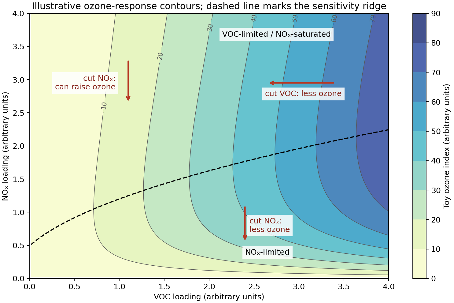
In an NOx-limited ozone-production regime, NO is too scarce for efficient peroxy-radical conversion; competing peroxide-forming radical termination becomes important. Reducing nitrogen-oxide emissions then reduces ozone production. In a VOC-limited ozone-production regime, plentiful nitrogen oxides remove OH through $\mathrm{OH}+\mathrm{N}{\mathrm{O}}_2+\mathrm{M}\to \mathrm{HN}{\mathrm{O}}_3+\mathrm{M}$, so organic oxidation and radical supply are limiting. Reducing volatile-organic emissions is effective there, while a modest nitrogen-oxide reduction can initially increase ozone by reducing radical termination and NO titration. Sufficiently large nitrogen-oxide reductions can move the system into the limited regime and eventually lower ozone. The appropriate control therefore depends on the chemical regime and the regional transport history, not merely the largest local emission. The ozone isopleth diagram below uses an explicitly schematic response function to show derivative signs, not a fitted concentration or emissions-control prediction.^[ref]

Lower winter temperatures favour formation and persistence of polar stratospheric clouds, providing particle surfaces on which reservoir chlorine can be activated, for exampleThese are heterogeneous surface processes; cooling changes particle abundance, adsorption, phase and reaction uptake, so a simple gas-phase Arrhenius argument is insufficient. Removal of nitric acid in sedimenting particles can also delay conversion of active chlorine back into chlorine nitrate. The relevant condensation thresholds depend on pressure and water/nitric-acid abundances, rather than a single universal temperature.

Once sunlight is present, $\mathrm{C}{\mathrm{l}}_2+\mathrm{h}\nu \to 2Cl$ provides active chlorine. In the chlorine monoxide dimer cycle,The net reaction is $2{\mathrm{O}}_3\to 3{\mathrm{O}}_2$, with chlorine regenerated. Low temperature favours formation of the ClOOCl dimer and suppresses its thermal dissociation, making photodissociation rather than thermal return of two ClO radicals more competitive. Laboratory flow experiments formed the dimer at 220–240 K and distinguished its infrared and ultraviolet signatures, supporting the chemical identity needed for this mechanism.^[ref]

Colder polar conditions can prepare and sustain greater springtime ozone loss, but darkness alone does not drive the photolytic cycle. In polar night reactive precursors can accumulate; sunlight is required for rapid dimer-cycle ozone destruction. This differs from the middle-stratospheric gas-phase cooling response derived above.^[ref]

Much stratospheric heating is supplied by absorption of solar ultraviolet radiation by oxygen and ozone, whereas carbon dioxide is an important emitter of thermal infrared radiation. In the usual stratospheric balance, increasing carbon dioxide enhances net infrared cooling at the original temperature without supplying a matching increase in the solar heating. Temperature must fall until infrared emission and absorption again balance the heating.

A useful optically thin schematic is $Q_{\mathrm{solar}}=c_{\mathrm{C}{\mathrm{O}}_2}K[B(T)-\overline{J}]$, where $B(T)$ represents the relevant thermal source function and $\overline{J}$ the incident infrared radiation field. With positive fixed solar heating and an approximately fixed radiation field, increasing $c_{\mathrm{C}{\mathrm{O}}_2}$ lowers the required $B(T)-\overline{J}$, hence lowers $T$. This explains why the surface greenhouse argument cannot simply be applied locally to the stratosphere. Spectral blocking of upwelling radiation contributes too; the real response depends on altitude, ozone heating and radiative transfer, rather than emissivity alone.^[ref]

Convert the molar mass to $0.0288\mathrm{kg}\mathrm{mo}{\mathrm{l}}^{-1}$ before substitution:The often-used environmental value near $-6.5\mathrm{K}\mathrm{k}{\mathrm{m}}^{-1}$ is less steep because rising moist air can condense water vapor, releasing latent heat and offsetting some expansion cooling. A saturated parcel therefore follows a smaller-magnitude moist adiabatic lapse rate, which varies with temperature, pressure and water content. Real environmental profiles also reflect radiation, mixing and weather systems; $6.5\mathrm{K}\mathrm{k}{\mathrm{m}}^{-1}$ is a representative profile value, not a universal parcel law.

Take a fixed amount of dry air, with no phase change, moving quasistatically so that its pressure matches the surrounding atmosphere. From the first law of thermodynamics and $H=U+pV$,For adiabatic motion $dq=0$. Treating the parcel as an ideal gas of fixed composition makes its enthalpy depend only on temperature, so for $n$ moles $dH=n{C}_{p}dT$ even though the pressure changes. Hence $n{C}_{p}dT=Vdp$. The environment is in hydrostatic equilibrium, $dp/dz=-\rho g$, and the parcel is taken to have the ambient density at the displacement point. Using $\rho =nM/V$ givesHere $C_p$ is molar and $c_p=C_p/M$ is mass-specific heat capacity. Positive $z$ points upward; the commonly quoted positive dry adiabatic lapse rate is ${\Gamma }_d=-dT/dz$. Approximate constancy of $g$ and heat capacity gives a constant gradient. Condensation, external heating, entrainment or composition changes invalidate this dry-parcel relation.

For a gas whose lifetime is much less than the selected horizon, the numerator of its global warming potential has nearly saturated: ${\int }_0^H{a}_i{m}_i(t)dt\simeq a_i{m}_i(0){\tau }_i$. The carbon-dioxide denominator continues to accumulate because of its long-lived response. Consequently a shorter horizon usually gives a larger GWP for this short-lived substitute; a longer horizon gives a smaller GWP. If the horizon becomes comparable to, or shorter than, the substitute's lifetime, the numerator also depends strongly on the horizon and cannot be replaced by its infinite-time limit.

The horizon is a value choice, and integrated forcing is not the same as temperature at a chosen future date. Equal-GWP pulses can therefore have different near-term warming and long-term temperature paths. The result also depends on greenhouse gas radiative efficiency, background concentrations, lifetime estimates and which indirect chemical effects or feedbacks are included. A pulse-based metric does not by itself describe a continuing emissions trajectory, nor does it measure ozone depletion or local air-pollution impacts. Comparisons should state the horizon, the emission scenario and the chosen climate outcome.^[ref]

TODO: user-deferred biological component. Biological carbon uptake, storage and release are outside the current scope. The physical and ocean-chemistry explanation is given here; the deferred component means this is not a complete all-process answer.

There is no single first-order atmospheric lifetime for an added carbon dioxide pulse. Air–sea gas exchange and adjustment of the surface mixed layer act on years-to-decades scales; redistribution into the ocean interior takes centuries to millennia. These transfers partition carbon between atmosphere and ocean rather than making the entire added carbon inventory disappear. Dissolution also changes the ocean's carbonate speciation: conversion among dissolved carbon dioxide, bicarbonate and carbonate buffers the uptake, but provides a finite capacity at a given alkalinity. A substantial perturbation therefore remains airborne after the faster exchanges have adjusted.

Further removal involves dissolution of carbonate sediments and carbonate compensation over several thousand years, followed by the much slower silicate-weathering and burial pathway, typically tens to hundreds of thousands of years. The exact fractions and times depend on pulse size and model conditions. A thousand years exceeds the fast exchange times but not the complete ocean–solid-Earth adjustment time, so a residual atmospheric perturbation is expected. An intercomparison found a substantial long tail after ocean equilibration, with further carbonate neutralization on roughly 3–7 kyr scales.^[ref]

The global warming potential compares equal-mass pulses, while the tabulated greenhouse gas radiative efficiencies are per ppb. For a fixed emitted mass, the initial mixing ratio is inversely proportional to molar mass. The molecular formulas give approximately $M_r=151.39\mathrm{g}\mathrm{mo}{\mathrm{l}}^{-1}$ for ${\mathrm{C}}_2{\mathrm{H}}_2\mathrm{C}{\mathrm{l}}_3\mathrm{F}$ and $M_{11}=137.36\mathrm{g}\mathrm{mo}{\mathrm{l}}^{-1}$ for $\mathrm{CC}{\mathrm{l}}_3\mathrm{F}$. Thus the ratio of mass-based greenhouse gas radiative efficiencies is $(0.24/0.26)(M_{11}/M_r)$.

In the standard one-box interpretation, the two quoted removal times represent independent first-order sinks acting on the burden. Their rates add, givingFor exponential pulse removal, the time-integrated abundance is proportional to $\tau (1-e^{-H/\tau })$. Dividing the replacement's forcing integral by the CFC-11 integral cancels the unknown carbon-dioxide reference integral:The finite-horizon factor for CFC-11 is important: $1-e^{-100/55}=0.8377$, not one. Omitting the molar-mass correction would incorrectly compare equal-ppb rather than equal-mass pulses.

This is about 76 times smaller than the stated CFC-11 value, because rapid tropospheric removal outweighs the fairly similar per-ppb greenhouse gas radiative efficiencies. It still represents appreciable warming per emitted mass. If the shorter lifetime alone is used as the troposphere-dominated approximation, the result is ${\mathrm{GWP}}_{100}\simeq 70.4$, close to the combined-rate result. If the two given lifetimes instead describe separate local compartments, an exact two-box calculation would also require exchange rates and burden partitioning; those are not supplied. The boxed result states the usual one-box assumption explicitly.