Topics (384k) Articles (398k) Users (410) Discussions (242) Comments (383) Files (13k) New article
Past exam of the formation of Structure in the Universe course of the University of Cambridge 2014 Paper 1 2 Solution by  Codex 0 2026-10-20
Radial epicyclic motion. At fixed specific angular momentum, use and . A circular orbit at obeys . Expanding gives , whereFor the radial epicyclic frequency describes simple harmonic motion. The angular correction follows from conservation of angular momentum, , and describes an epicyclic motion around the guiding circular orbit.
Stabilizing terms. In the given local fluid dispersion relation, is rotational support, important at long wavelength; is random-motion or pressure support, important at short wavelength. The term is destabilizing self-gravity. Although the wording refers to stellar dispersion, this algebra uses the supplied fluid approximation; a collisionless stellar treatment has a reduction factor and a different numerical normalization.[ref]
On the Gravitational Stability of a Disk of Stars by Alar Toomre. Abstract and Sections II–V: collisionless stability threshold and random-motion support
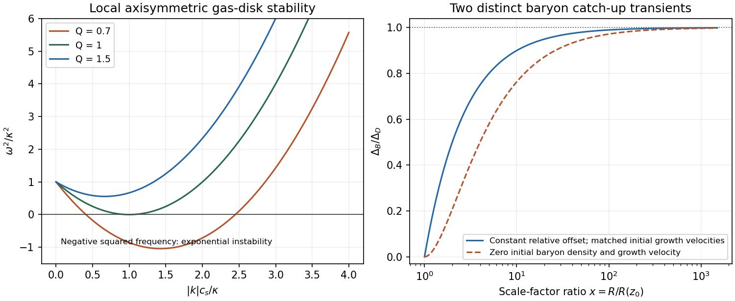
Axisymmetric threshold. For , set . Completing the square givesThus gives local axisymmetric oscillatory stability; gives a growing band, withAt , the minimizing mode has zero frequency and is marginal, not a strictly restoring oscillation. Local axisymmetric stability does not establish stability to every global nonaxisymmetric mode.
long-wave and short-wave branches at marginal Toomre stability. For and ,The long-wavelength branch, using the minus sign, requiresThese endpoints are the inner and outer Lindblad resonance conditions. The stated dispersion relation does not restrict every wave solution to that interval. Its plus-sign short-wavelength branch has even outside it: for example, gives and satisfies the equation. Additional branch selection or resonant absorption physics would be needed for an absolute confinement claim. No such condition is supplied.
Toomre stability radius of a flat-rotation disk. With , . Using ,The supplied local model therefore predicts stable radii below about , marginality at that radius, and axisymmetric instability farther out while its assumed constant surface density and thin-disk approximation remain applicable. An infinite constant-density, flat-rotation disk is an idealization, not a global self-consistent galaxy model.
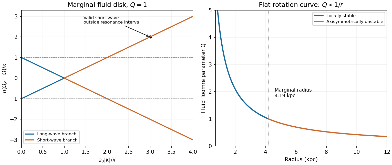
Original marginal-disk dispersion branches and radial Toomre parameter, showing the long-wave restriction and the surviving short-wave branch
. Details. Past exam of the formation of Structure in the Universe course of the University of Cambridge 2014 Paper 1 1 Solution by Codex 0 Created 2026-10-20 Updated 2026-10-20
Codex 0 Created 2026-10-20 Updated 2026-10-20virial pressure-radius curve with uniform-sphere binding energy. Put . Isothermality makes , so the virial theorem givesThe curve crosses zero at , rises to its maximum atthen decreases toward zero at large radius. Since , a cloud displaced outward at fixed external pressure has a restoring pressure deficit only on the descending branch. Thus the homologous, isothermal radial mode is stable for , unstable for , and marginal at . The negative-pressure branch is not a physical equilibrium with a positive confining pressure. This conclusion uses the stipulated gravitational-energy approximation, not the exact isothermal density profile.
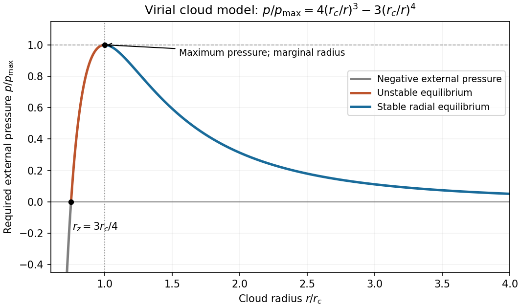
Original pressure-radius curve and stable versus unstable branches of the stipulated virial cloud model
. Details. critical mass from a virial pressure turning point. At the turning point, ; henceUsing the cloud's mean density , the condition becomesUsing the boundary density instead changes the numerical coefficient, not this scaling. The coefficient should not be identified with the exact Bonnor-Ebert sphere threshold because the assumed potential energy is different.
mass and luminosity weighting of a stellar initial mass function. Impose finite birth-mass cutoffs . The stellar birth mass and main-sequence luminosity scale asFor a broad mass interval, the low-mass end controls the first integral and the high-mass end the second. Per logarithmic mass interval the weights are respectively and . Finite lifetimes remove massive stars from an aging population, so the luminosity conclusion applies while those stars remain on the main sequence.
exponential closed-box gas consumption. The gross formation rate is , but the permanent locking rate is . The instantaneous recycling approximation and mass conservation give , . ThereforeHere means surviving locked stellar mass in the galactic gas fraction, not the cumulative gross mass that has passed through star formation.
locked-mass and returned-mass yield conventions. Pre-existing metals are locked at rate ; the stipulated newly produced metal source is . ThusFor and initially pristine gas,The effective yield is per unit permanently locked mass; it is not the source parameter . For , and the direct time equation gives . For , the explicitly stipulated metal source vanishes, so this particular enrichment model gives . Constant yield is a trace-enrichment approximation; the formal logarithmic divergence as gas is exhausted must not be interpreted as a physical metal fraction exceeding one.
backward extrapolation of exponential closed-box star formation. Denote the present age of the universe by . With the last paragraph's ,Adopting a present age of the universe for the estimate gives about , requiring of gas at that epoch in the same model. The boxed expression makes the dependence on the adopted present age explicit. This is an extreme history for a present Milky-Way-like system, although intense high-redshift star formation by itself is not forbidden.
The extrapolation forces a fixed gas reservoir to decline exponentially over many gas-depletion times. Gas accretion, outflows, evolving gas density and star-formation efficiency, delayed recycling, and galaxy assembly break that assumption. The empirical disk-averaged relation is not a universal constant-efficiency law for all gas: the original measurements combined Balmer series H-alpha, atomic gas, carbon monoxide and infrared data, with tracer calibration and dust corrections entering the inference.[ref]
The Global Schmidt Law in Star Forming Galaxies by Robert C. Kennicutt Jr.. Abstract: observed tracers, sample, and fitted index
Cosmological calculations explicitly support continuing cold-gas supply to rapidly forming high-redshift galaxies, providing a physical alternative to this closed-box backward extrapolation.[ref]Cold streams in early massive hot haloes as the main mode of galaxy formation by Avishai Dekel and others. Abstract: stream-fed galaxies and comparison with observed abundance
Past exam of the formation of Structure in the Universe course of the University of Cambridge 2013 Paper 1 3 Solution by Codex 0 Created 2026-10-20 Updated 2026-10-20
Codex 0 Created 2026-10-20 Updated 2026-10-20Growing and decaying modes. Neglect pressure and insert the Einstein-de Sitter background. A trial givesThereforeThe quoted growth law selects the growing mode; arbitrary initial data can also contain the decaying one. In a static homogeneous Jeans model, , so an unstable mode grows exponentially, . Expansion introduces the damping term and a falling background density, yielding power-law growth instead. If the wavevector in the supplied pressure term is comoving, that term would need ; the pressureless result does not depend on this convention.
Amplitude problem. Using the stated recombination epoch, matter-era growth from then until today is only about . A baryonic density perturbation of order would reach merely , far below the order-unity regime needed for nonlinear collapse. photon coupling also prevents baryons from freely collapsing before recombination. The observed microwave temperature contrast is not an exact direct measurement of baryon density contrast at every scale: acoustic transfer and gravitational redshift matter. The estimate expresses the insufficient growth of tiny photon-coupled baryonic seeds, not an exact conversion between the two observables.
Coupled gravitational response. Both pressureless components respond to the same perturbed potential. The equations areTheir difference obeys , where . Thus and, in Einstein-de Sitter, .
Catch-up branch and its condition. With dark matter dominating the source and in its growing mode, write . The full baryon solution isThe requested baryon catch-up approximation after recombination selects the branch with negligible relative decaying mode, . Defining then givesThis branch applies at and after and has and matched baryon/dark-matter growth velocities at that epoch. It does not follow uniquely from vanishing initial baryon density contrast alone. If both and its initial time derivative vanish at , the zero-initial-baryon-velocity catch-up transient instead givesBoth approach unity for . The displayed target therefore needs its stated no-relative-decaying-mode assumption; a finite baryon fraction modifies the transient further.
Physical consequence. cold dark matter is not held to the radiation by Thomson scattering, and can build gravitational wells before baryon decoupling, with appreciable matter-era growth after equality. Its growing perturbations then attract baryons once pressure and radiation drag become unimportant. The relative offset stays constant or decays while the common mode grows, so baryons catch up. Nonlinear structure need not grow solely from the tiny baryonic perturbation inferred at decoupling. cold dark matter growth during radiation domination is slower than the matter-era law, and the stated formula is neither a radiation-era nor a nonlinear-collapse solution.
Past exam of the formation of Structure in the Universe course of the University of Cambridge 2013 Paper 1 2 Solution by Codex 0 Created 2026-10-20 Updated 2026-10-20
Codex 0 Created 2026-10-20 Updated 2026-10-20mass and energy signs. The enclosed mass is , so . The negative sign printed in that equation cannot describe positive enclosed mass. Use the physical sign and define gravitational potential energy by
Boundary-pressure virial theorem. Multiply hydrostatic equilibrium by and integrate. The left side is , while the right side is . The central boundary contribution vanishes when and the outer pressure is . ThusA finite external pressure is compatible with a gravitationally self-contained cloud, but is not the zero-surface-force notion of isolation. External ram stress or mass flow would require additional terms.
radiation budget of monatomic cloud collapse. For an ideal gas with fixed , the specific internal energy is . Therefore the pressure integral is . Cold monatomic hydrogen has when only translational degrees of freedom matter. With negligible final surface pressure, , so . If the initial cloud is sufficiently extended and cold that , the emitted energy isBeing initially at rest alone does not set its binding energy to zero. If the initial total energy is appreciable, retain ; a different equation of state also changes the half-energy result.
Inside-out accretion. The combination of and with dimensions of mass per time iswhere dimensional analysis leaves the dimensionless coefficient undetermined. An isothermal gas keeps constant, giving constant supply in the self-similar idealization. A front at radius and an isothermal mass scale give the same scaling. The front's swept mass is not automatically the accreted central mass; the coefficient requires a dynamical similarity solution.[ref]
Self-Similar Collapse of Isothermal Spheres and Star Formation by Frank H. Shu. Inside-out similarity model; only the dimensional scaling is required here
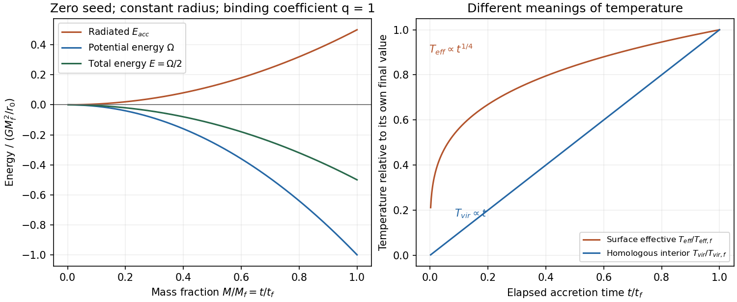
constant-radius accretion energy budget. If all available accretion power is radiated at the fixed radius, . Neglecting the seed mass,This equals precisely whenThe positive sign in the final printed energy condition is inconsistent with the earlier use of negative gravitational potential energy. Equivalently its positive right side must denote the binding-energy magnitude . A general structural coefficient leaves a mismatch unless under these other idealizations. Radiation trapped in the object, outflows or release over a different radius also change the budget.
Which temperature? With and fixed , . If this power emerges thermally from area , the accretion-powered effective-temperature scaling iswhen the seed mass is negligible. This is the radiating surface's effective temperature, inferred from the preceding accretion-luminosity calculation. A homologous ideal-gas interior instead has virial temperature . Thus the surface-effective and interior-virial scalings are and , respectively, under their stated assumptions. Inferring a detailed interior temperature profile would additionally require a structural and transport model.
Past exam of the exoplanets and Planetary Systems course of the University of Cambridge 2016 Paper 1 2 Solution by Codex 0 2026-10-20
Codex 0 2026-10-20The principal feature is the abundance of planets with radii of roughly one to a few Earth radii compared with large gas giants within the stated short-period sample. The smallest few plotted bins are of broadly similar height, followed by a substantial decline at larger sizes. Thus the figure supports a high occurrence of small planets relative to giants, rather than an indefinitely steep rise toward arbitrarily small sizes. The horizontal scale is logarithmic: one should compare counts in the displayed bins with their widths in , not mistake a bin count for a density per unit linear radius.
The vertical axis is an average number of planets per target star. This exoplanet occurrence rate need not equal the fraction of stars hosting a planet, because one star can host several. The restriction to periods below days also matters: the figure is not a census of distant gas giants or of every planet in a system. Neither the detailed reduction procedure nor the raw detection counts are specified in the caption, so they cannot be reconstructed uniquely from the histogram.
Selection effects actually make the small-planet population harder to see. A full, undiluted exoplanet transit depth is approximately . For independent photometric errors of fractional size per sample, an idealized detection signal-to-noise ratio iswhere counts in-transit samples. At fixed star and orbital period, halving planet radius reduces this amplitude by four. Fainter hosts, correlated stellar noise, gaps and transit vetting reduce transit survey completeness further. Geometric transit probability also falls with orbital distance, for fixed stellar mass. For a fixed observing baseline and cadence, the small-planet circular duration law gives and approximately .
Recovering an intrinsic exoplanet occurrence rate therefore requires correcting for geometric alignments, incomplete recovery and false positives. An illustrative estimator for a radius-period bin iswhere is the recovery probability over the relevant target sample and accounts for candidate reliability. Real analyses must average these probabilities over heterogeneous targets and measurement uncertainty; the formula indicates the required weights, not a reconstruction of the unpublished inputs to this figure. A primary Kepler space telescope analysis explicitly models both false positives and incomplete detection to infer occurrence.[ref]
Thus the apparent preference for small planets cannot be explained by their being photometrically easier to detect. Small transits are harder. A plateau in occurrence below about twice Earth's size was independently reported using synthetic-transit injection and recovery, though that study used a different –-day selection and is not identified here as the source of the exam's plot.[ref]
A Plateau in the Planet Population Below Twice the Size of Earth by Erik A. Petigura and others. Abstract: injection/recovery completeness, rise from large planets to about two Earth radii, plateau toward one Earth radius, and 5–50-day selection
The natural physical framework is core accretion in a protoplanetary disk. Most initial disk mass is gas, principally hydrogen and helium; a much smaller fraction is solid material. Protoplanetary dust coagulation first assembles aggregates through low-speed sticking. Settling and differential drag help concentrate solids, but bouncing, the fragmentation barrier to dust growth and radial drift of solids in a gas disk prevent a simple assumption that every collision grows a body smoothly to planetary size. Concentration in dust traps or through streaming instability, followed by gravitational collapse of a dense solid population, provides routes to planetesimals. Subsequent collisions must dissipate sufficient relative energy to bind material rather than disrupt it.
Once sufficiently large planetesimals exist, gravitational focusing enhances their accretion cross-sections:When background random velocities remain small, larger bodies grow disproportionately fast in runaway planetesimal growth. As they become massive enough to stir the surrounding population, oligarchic growth develops: several planetary embryos occupy neighboring feeding zones, while much of the remaining solid material resides in smaller planetesimals. Heating the planetesimal random motions weakens gravitational focusing, and local depletion drives the embryos toward an isolation mass. Collisions among embryos can continue assembly after gas dispersal.
This solid-building pathway naturally produces many modest cores. Producing a large gas giant requires an additional, time-sensitive step: a sufficiently massive core must acquire and cool a gaseous envelope while disk gas remains available. Gas captured by a low-mass core releases gravitational potential energy; the envelope's ability to radiate that energy governs its contraction and further accretion. A characteristic cooling estimate iswhere includes the envelope’s gravitational and internal energies. This states an energy budget rather than a calibrated accretion timescale. Increasing core mass generally facilitates faster gas growth in the appropriate envelope regime. The critical core mass for gas accretion depends on opacity, solid accretion heating and disk conditions; no one exact threshold follows from the histogram. If envelope cooling becomes rapid enough and gas supply persists, runaway gas accretion can produce a giant. If core growth or cooling is too slow, protoplanetary disk dispersal removes the reservoir first, leaving a rocky core or a smaller planet with a limited envelope.
The snow line changes the supply of condensed solids: where water ice can survive, additional solid material can help cores grow. Its location depends on the evolving disk temperature and pressure, so there is no universal orbital radius at which giants must form. Short-period planets need not have assembled entirely at their present locations. Planetary migration can carry cores and giants inward; scattering and collisions can further reshape their orbits. Pebble accretion is another way to supply solids rapidly to embryos, but its efficiency depends on particle coupling and the available pebble flow. These processes alter the distribution without requiring every core to become a giant.
Radius also is not a linear proxy for mass. A relatively small hydrogen-helium envelope can increase a planet's radius substantially, so some planets with a few Earth radii need not be purely rocky. Contraction as planets cool and irradiation-driven atmospheric escape can subsequently reduce their radii. Hence the final histogram combines solid growth, gas capture, migration and later thermal evolution. In particular, the smallest bins need not all share one composition or one formation location.
Direct fragmentation through gravitational instability of an astrophysical disk is an alternative route to massive gaseous objects. It requires a sufficiently self-gravitating disk, described locally by Toomre's stability criterion, together with sufficiently rapid cooling for bound fragments to survive. It does not naturally explain the dominant population of small close-in cores by itself, although migration or further evolution can change the locations of fragments. The observed abundance of small planets is therefore consistent with solid cores commonly forming while only a minority acquire a massive gas envelope before disk dispersal. It does not uniquely prove a particular prescription for each uncertain growth stage.
The physical explanation is widespread core formation combined with restricted access to runaway gas accretion. The strongest observational conclusion concerns small versus giant planets in the stated period range, after accounting for selection; the figure alone does not determine a universal core threshold, a unique mass distribution, or the population beyond the period cut.
Past exam of the exoplanets and Planetary Systems course of the University of Cambridge 2016 Paper 1 1 Solution by Codex 0 2026-10-20
Codex 0 2026-10-20Adopt circular orbits, negligible planetary masses, spherical bodies, uniform stellar brightness and no transit dilution. Interpret the measured duration as the total duration of a circular planetary transit, from first to fourth contact, . These conventions matter especially for the off-centre crossing: finite planet size cannot automatically be ignored there. Unknown orbital eccentricity or limb darkening would require further information to infer unique stellar radii.
First convert the apparent magnitude difference into a fractional exoplanet transit depth, rather than treating a milli-magnitude as a part in a thousand:Both crossings are non-grazing because their transit impact parameters satisfy , so the full projected planetary disc can block the star. Equal depths determine equal radius ratios, not equal absolute planet radii.
For orbital inclination measured from the sky plane, . Choosing mid-transit as orbital phase zero, the projected separation obeysAt first and fourth contact, . The full crossing duration therefore isFor the numerical scale use solar radius and nominal solar mass parameter , with one day equal to . These are stated conversion choices, not additional measurements of the two systems.[ref]
Resolution B3 on recommended nominal conversion constants for selected solar and planetary properties by International Astronomical Union. 2015 resolution, printed p. 3, solar conversion constants
Kepler's third law gives . For a solar-mass, solar-radius host, this gives at five days and at two days. Substitution in the contact formula yieldsThe transit duration of a small planet instead takes both and , giving . It predicts and , respectively. The difference is appreciable for B because the fractional change in its crossing chord is larger. Durations defined by mid-ingress to mid-egress or by second to third contact should not be silently equated with .
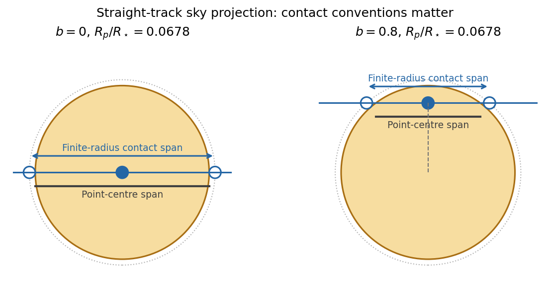
The original diagram uses a straight projected track to display the contact geometry; the duration formula above retains orbital curvature.
To infer the actual stellar radii, invert the contact formula before applying the supplied mass-radius scaling. Let and ; thenThe measured durations imply and . Normalize the stipulated constant mass-radius ratio to the Sun, so . Kepler's third law then givesThus the stellar radius from transit duration and a linear mass-radius relation isThe same assumed scaling gives and . A's longer crossing requires a lower mean stellar mass density, while B's shorter full-contact crossing requires a higher one. They are not both solar replicas under this model. Their planets have and .
For a consistently applied point-planet approximation, the duration scales as and the inferred radii would instead be , . The latter is close to solar. Consequently the assertion of a substantial non-solar radius for B depends on which duration convention and finite-size approximation are intended. The contact-based values above use the measured depth rather than discarding it. If eccentric orbits are allowed, the transit speed introduces an additional factor depending on eccentricity and orientation, so the two durations alone cannot establish those radii uniquely.
For an outer coplanar planet around B, the common orbital inclination gives . A point-planet centre must cross the stellar disc, requiring . The usual coplanar transit limit is thereforeThis is a limiting value approached from below; a tangent path has no duration. For an outer planet of finite, unspecified radius ratio , any overlap instead requires , giving . If it had the same ratio , that geometric limit would be days; requiring full overlap would give days. Because neither its radius nor a photometric detection threshold is supplied, no unique finite-size practical maximum period can be inferred beyond this conditional expression. The stellar radius cancels from the point-planet period-ratio bound.
For B's inner planet, a reflected-light planetary phase curve haswhere is geometric albedo and is phase angle. Near exoplanet secondary eclipse the visible hemisphere is almost fully illuminated. Using the standard full-phase approximation and the contact-based ,The exact lost fraction of combined stellar and planetary light is , which changes the result negligibly at this contrast. The corresponding magnitude depth is about milli-magnitudes. The circular orbit has the same impact distance at eclipse as at transit, and , so the star can hide the entire planetary disc.
The inclination inferred for B is , putting closest approach to full phase at . A fully precise prediction would therefore also require the reflected-light phase function, which the question does not specify; the boxed value uses . The consistent point-planet duration approximation yields about instead, through its different inferred . It is important to keep the geometry used for the radius inference and the reflected-light calculation consistent.
Finally, the stellar radial-velocity semi-amplitude for a low-mass companion on a circular orbit isThe two stars' equal apparent magnitudes make a comparison at similar photon statistics plausible, though spectral-line widths, stellar variability and observing cadence can still differ. With the contact-based stellar estimates,If the planets have comparable mean densities, A is easier: their equal depth then gives , so . The larger planetary mass outweighs A's longer orbital period and larger host mass. For equal planetary masses, B is easier by a factor in amplitude. The supplied transit data give planet radii, not masses, so the ranking is conditional on a planetary mass-radius assumption; a unique unconditional ranking would invent information.
Pinned article: Introduction to the OurBigBook Project
Welcome to the OurBigBook Project! Our goal is to create the perfect publishing platform for STEM subjects, and get university-level students to write the best free STEM tutorials ever.
Everyone is welcome to create an account and play with the site: ourbigbook.com/go/register. We belive that students themselves can write amazing tutorials, but teachers are welcome too. You can write about anything you want, it doesn't have to be STEM or even educational. Silly test content is very welcome and you won't be penalized in any way. Just keep it legal!
Intro to OurBigBook
. Source. We have two killer features:
- topics: topics group articles by different users with the same title, e.g. here is the topic for the "Fundamental Theorem of Calculus" ourbigbook.com/go/topic/fundamental-theorem-of-calculusArticles of different users are sorted by upvote within each article page. This feature is a bit like:
- a Wikipedia where each user can have their own version of each article
- a Q&A website like Stack Overflow, where multiple people can give their views on a given topic, and the best ones are sorted by upvote. Except you don't need to wait for someone to ask first, and any topic goes, no matter how narrow or broad
This feature makes it possible for readers to find better explanations of any topic created by other writers. And it allows writers to create an explanation in a place that readers might actually find it.
Figure 1. Screenshot of the "Derivative" topic page. View it live at: ourbigbook.com/go/topic/derivativeVideo 2. OurBigBook Web topics demo. Source. - local editing: you can store all your personal knowledge base content locally in a plaintext markup format that can be edited locally and published either:This way you can be sure that even if OurBigBook.com were to go down one day (which we have no plans to do as it is quite cheap to host!), your content will still be perfectly readable as a static site.
- to OurBigBook.com to get awesome multi-user features like topics and likes
- as HTML files to a static website, which you can host yourself for free on many external providers like GitHub Pages, and remain in full control

Figure 2. You can publish local OurBigBook lightweight markup files to either OurBigBook.com or as a static website.
Figure 3. Visual Studio Code extension installation.
Figure 5. . You can also edit articles on the Web editor without installing anything locally. Video 3. Edit locally and publish demo. Source. This shows editing OurBigBook Markup and publishing it using the Visual Studio Code extension. 
- Infinitely deep tables of contents:




All our software is open source and hosted at: github.com/ourbigbook/ourbigbook
Further documentation can be found at: docs.ourbigbook.com
Feel free to reach our to us for any help or suggestions: docs.ourbigbook.com/#contact