Topics (384k) Articles (398k) Users (410) Discussions (242) Comments (383) Files (13k) New article
Past exam of the frontiers of Observational Astrophysics course of the University of Cambridge 2014 Paper 1 2 Solution by  Codex 0 2026-10-20
The observed population is the parent population filtered by an astronomical selection function and measurement errors. Malmquist bias arises because a flux-limited galaxy selection admits luminous objects from larger volumes: in Euclidean space and . Thus observed luminosity counts are weighted by . Even a nominal standard candle with intrinsic scatter is preferentially observed on its bright side near the limit; ignoring this can underestimate distances. A volume-limited sample or a justified weighting helps, subject to completeness, geometry and evolution assumptions. Separately, Eddington bias occurs when noise scatters a steeply rising population across a detection threshold: more faint objects enter than bright objects leave.
Lutz-Kelker bias concerns noisy stellar parallaxes and population/selection weighting. Locally uniform spatial density gives and, by changing variables, over the model's valid finite range. More distant stars are available to scatter into a parallax-limited sample than nearby stars to scatter out. Inverting an uncertain parallax also introduces a distinct nonlinear-estimation problem. There is no universal magnitude correction for every star: spatial density, luminosity, extinction and how the sample was selected all matter. The classical treatment motivates this issue; it should not replace an explicit generative model.[ref]
On the Use of Trigonometric Parallaxes for the Calibration of Luminosity Systems: Theory by T. E. Lutz and D. H. Kelker. PASP 85, 573–578; classical uniform-density calibration model
Bayes' theorem combines the measurement likelihood function with a justified prior distribution. For example, with a Gaussian parallax error and consistent distance/parallax units,A proper distance prior for parallax inference might have with a justified scale ; extending to infinity gives an improper posterior here. Negative measured parallaxes remain valid noisy data. For selection conditioning in Bayesian inference, distinguish individual inference from population inference: if selection is determined entirely by the exact data already conditioned on, it adds no further information about that individual's parameters. For population parameters , the selected-data likelihood must instead include the detection normalization . Applying a cut twice is also an error.
Selection can depend on surface brightness, angular resolution, dust, sky coverage, colour and observing cadence as well as total flux. Crowding and unresolved binaries bias distance calibrators. Transit surveys favour large planets and short periods, with an additional geometric transit probability approximately for small planets on circular orbits; injection/recovery tests quantify the remaining transit survey completeness. Cluster catalogues select noisy mass proxies from a steep abundance distribution. Planck's 2013 SZ catalogue explicitly characterized detection completeness and reliability rather than identifying every detection with an unbiased mass census.[ref]
Planck 2013 results. XXIX. Planck catalogue of Sunyaev-Zeldovich sources by Planck Collaboration. abstract and selection-function/completeness analysis, 2013 preprint
Calibrators, artificial-source tests and a forward model of detection, measurement and follow-up are the practical checks on any correction. Past exam of the frontiers of Observational Astrophysics course of the University of Cambridge 2014 Paper 1 1 Solution by Codex 0 2026-10-20
Codex 0 2026-10-20The detector is intended for arcsecond-scale astronomical seeing, rather than the telescope's diffraction limit. A circular aperture of this area has diameter , giving a Rayleigh criterion angle about arcsec at the observing wavelength. One-arcsecond pixels conventionally sample an astronomical seeing profile of roughly two arcseconds across with two samples; a one-arcsecond profile would be undersampled. The pixel scale alone does not determine an exact astronomical seeing width.
Use the supplied surface brightness as radiative flux integrated over the photometric passband: its units contain no inverse hertz. Treat as the representative photon energy, and assume unit throughput and quantum efficiency. A genuinely frequency-specific brightness would require a bandwidth. With angles measured consistently in arcseconds, an annulus has area square arcseconds, soThis is flux per collecting area; collected energy is . There is no extra conversion to steradians when both brightness and angular area use square arcseconds.
For Poisson photon counting, a pixel with expected count has energy and standard deviation . Thus the local four-sigma rule gives , or 16 photons at the boundary. With pixel area ,Consequently arcsec andIntegrating to the model's outer radius arcsec instead givesThe pixel cut retains 51.6% of this total. It is an imposed isophotal photometry rule, not a fundamental limit: averaging annuli or fitting a justified profile can recover signal below the per-pixel cut.
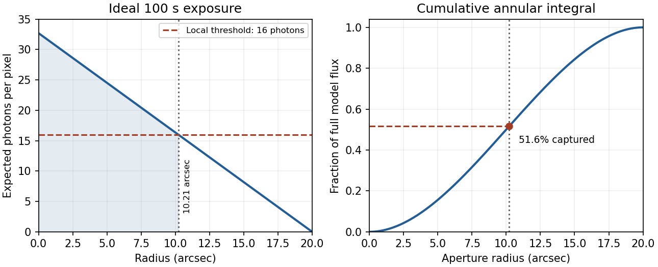
In practice, sky background photons add shot noise even after subtraction of the mean sky. read noise, dark current, imperfect flat-field correction, throughput calibration and atmospheric extinction also matter. At large radius the dominant uncertainty can be a tiny error in the sky level, scattered light or the wings of the point spread function, rather than source photon statistics. Mask foreground stars and background objects, compare blank-sky regions and dithered exposures, and check profile recovery by inserting artificial extended sources. astronomical seeing and finite pixels convolve the intrinsic profile; model that response when extrapolating the total.
The luminosity convergence of an outer surface-brightness profile follows directly: contributes , hence at large radius for . For either shallow index considered, ever larger annuli dominate: extending the law to infinity gives an unphysical divergent luminosity. Such a law must eventually steepen or truncate. Over a finite range, however, substantial light can lie below a surface-brightness selection threshold and be mistaken for sky. This biases galaxy luminosities, the luminosity function and the inferred diffuse light budget; distant diffuse galaxies become especially incomplete because bolometric cosmological surface-brightness dimming scales as . An assumed finite-aperture total is therefore a model-dependent quantity.
Past exam of the frontiers of Observational Astrophysics course of the University of Cambridge 2013 Paper 1 2 Solution by Codex 0 2026-10-20
Codex 0 2026-10-20The wavelength is . Thirty dishes give interferometric baselines. The longest projected baseline sets the finest angular scale, while the individual dish beam sets the instantaneous field of view. At the maximum separation,A aperture instead has primary-beam width of order , about arcseconds; the Airy first-null convention gives about arcseconds. Illumination taper changes the precise beam definition. The array therefore resolves many synthesized beams within one pointing, but it does not image an arbitrarily wide field at that resolution.
The shortest useful baseline determines missing large-scale structure. A common estimate is . If dishes can be packed with usable center separations near , this is of order arcseconds. A more extended layout has a smaller recoverable scale. The site diameter does not specify or the actual Fourier coverage, and low-elevation shadowing can remove short spacings. Mosaicking expands sky coverage but does not supply all zero-spacing information; suitable total-power or compact-array data help recover extended emission. Earth rotation and reconfiguration improve sampled baseline coverage, sidelobes and image reconstruction, with a tradeoff between resolution and surface-brightness sensitivity.
For dish aperture efficiency , . The system-equivalent flux density of one dish isFor independent receivers, natural weighting, correlator efficiency and equally sensitive polarization products contributing to intensity, the unresolved-source thermal rms isHere is usable bandwidth and integration time. A numerical sensitivity is therefore conditional on these unspecified observing choices. For an illustrative bandwidth, one hour, two polarizations and , it is about , or at . Resolved-source brightness sensitivity also depends on beam area and missing flux. The sensitivity expression assumes naturally weighted data and the stated polarization convention.[ref]
Earth rotation changes geometric delay. At a baseline , can be of order , here , and a raw fringe-rate bound isThe actual rate depends on geometry and source direction. Correlator delay tracking and fringe stopping compensate the chosen phase center rather than averaging rapidly rotating uncorrected fringes away. Off-center directions retain residual delays and rates.
Finite bandwidth causes chromatic phase averaging and radial bandwidth smearing. A direction offset has residual delay of order ; a channel should satisfy for small decorrelation. Across a field of order radians on the longest baseline, the one-cycle frequency scale is about , so substantially narrower channels are required for accurate wide-field imaging. Similarly, time averaging should keep ; the associated one-cycle scale is about seconds in this example. Frequency-resolved visibilities and shorter dumps control these field-dependent averaging losses in radio interferometry; they are averaging losses, not ordinary glass-lens chromatic focusing.
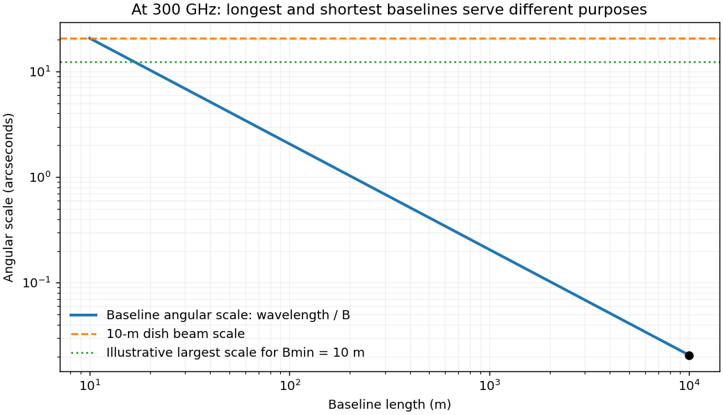
Millimeter-array baseline tradeoff: angular resolution and the loss of large-scale structure
. Details. At , atmospheric water vapor produces absorption, thermal emission and path-length fluctuations. A high dry site reduces these effects, while phase fluctuations can still destroy coherence on long baselines. A one-radian phase corresponds to path fluctuation , motivating frequent phase calibration or atmospheric path monitoring. Surface errors must also be small relative to the wavelength: the Ruze efficiency factor is . Pointing errors matter relative to a primary beam only tens of arcseconds wide.
Important systematic errors include antenna gains and bandpasses, delay and baseline-coordinate errors, polarization leakage, pointing, atmospheric opacity, correlator response and flux-scale calibration. Nearby compact calibrators, bandpass standards, appropriate total-power information and repeated configurations address different parts of this problem. High nominal collecting area and longest-baseline resolution alone do not determine image dynamic range or reliable extended-source flux.
Past exam of the frontiers of Observational Astrophysics course of the University of Cambridge 2013 Paper 1 1 Solution by Codex 0 2026-10-20
Codex 0 2026-10-20Bayes' theorem relates a model parameter and observed data by . The posterior describes the parameter after observation, the likelihood describes the data for a specified parameter, the prior describes the parameter before these data, and the evidence normalizes the posterior. Likelihood is a function of the unknown parameter; it is not automatically a normalized probability density over that parameter.
Stellar parallax is the apparent annual change of a nearby star's direction relative to distant background objects as the observer moves around the Sun. The conventional parallax angle uses a one-AU baseline, so in radians, or in parsecs and arcseconds. Many small approximately independent centroiding and reference-frame errors can yield approximately Gaussian parallax errors through the central limit theorem. Correlated calibration errors, outliers and low-signal image fitting can violate that approximation; Gaussian measurement errors also need not produce Gaussian errors after taking a reciprocal distance.
For a locally uniform spatial population, the number in a spherical shell is proportional to . Changing variables using givesThis is a local population-density rule on its valid distance range. It needs a finite population or survey boundary to be a normalized global prior. An unbounded volume prior combined with a Gaussian parallax likelihood can otherwise yield an improper posterior, as explained by the proper distance prior for parallax inference.
For the requested top-hat calculation, distinguish the unknown true parallax from the reported likelihood center . Take a known fixed half-width , so the likelihood is constant over . Assume this interval lies inside the applicable population range. The top-hat parallax posterior under a uniform-volume prior is thenSetting givesThe greater available volume at smaller true parallaxes weights that side of the likelihood more strongly. This inference is not an additional measurement of the star's actual parallax.
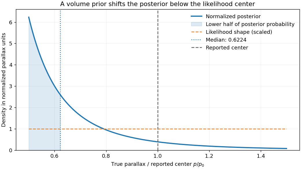
The printed notation uses both for the unknown true parallax and for the top-hat center in the numerical comparison. The distinct notation above states the consistent fixed-width interpretation yielding its result. If the half-width instead varies with the unknown parameter as , the normalized likelihood has an additional factor and different support; the same posterior calculation cannot be reused unchanged.
To improve distance inference, use independent information on luminosity, spatial density, extinction and sample selection. If the common luminosity in the measured band is calibrated, a flux measurement supplies another distance constraint through . If that common luminosity is unknown, it can be treated as a population parameter rather than silently assumed known. A finite distance distribution and the actual selection function specify which prior is appropriate. The classical Lutz-Kelker bias is a sample-calibration problem; a posterior shift under a justified prior is not itself an error to remove by a universal correction.
With flux-limited selection for identical standard candles and a noise-free threshold, there is a maximum observable distance, hence a minimum true parallax. The selected prior is truncated there. There is no luminosity-preference Malmquist bias if every object truly has the same luminosity. With a luminosity distribution, the accessible Euclidean volume scales as , preferentially including brighter objects; this is the Euclidean accessible-volume luminosity weighting underlying Malmquist bias. Flux errors additionally scatter numerous faint sources upward across a threshold, biasing selected measured fluxes. Extinction, different spectral energy distributions in a selection band, crowding, completeness and parallax-quality cuts can alter the effective population. These effects require a joint selection and error model rather than a single blanket parallax correction.
Past exam of the frontiers of experimental condensed matter physics course of the University of Cambridge 2013 Paper 1 3 Solution by Codex 0 2026-10-20
Codex 0 2026-10-20Atomic force microscopy senses tip–sample interactions through a compliant cantilever. Contact deflection, oscillation amplitude, phase or resonance frequency can be converted into a feedback signal. Chemical bonding and short-range repulsion, van der Waals forces, electrostatic forces and, where relevant, magnetic or capillary interactions produce contrast. Apparent height at a fixed force or frequency setpoint can therefore contain interaction contrast as well as geometry. Lateral resolution depends on the effective tip apex and interaction range; finite tip radius broadens features. Vertical sensitivity also depends on thermal and detector noise, cantilever calibration, vibration, drift and feedback bandwidth. Strongly localized short-range forces favor atomic resolution, whereas extended interactions average over more of the tip and surface.
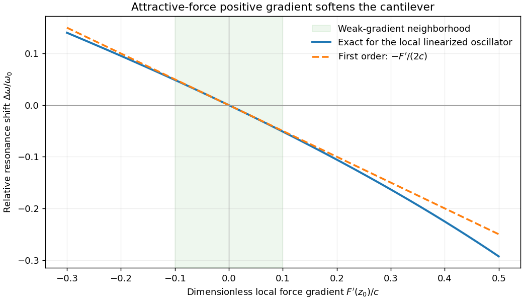
For small oscillations about equilibrium separation , write and linearize . The constant force is absorbed into the equilibrium displacement. The cantilever equation becomesConsequently the small-amplitude AFM frequency shift isThe linear expression is the small-force-gradient approximation, , in addition to the small-oscillation assumption. For an attractive force , and the resonance softens. A finite oscillation amplitude samples a weighted range of forces rather than only the gradient at one separation, and destroys local stability in this simple static model.
In a scanning electron microscope, a focused electron beam scans the surface and a detector records an emitted signal at each beam position. Low-energy secondary electrons escape from near the surface; changes in local slope, edges and detector-facing geometry give strong secondary-electron topographic contrast. Backscattered electrons result from elastic deflection of primary electrons and generally have a larger yield for higher atomic number. Their backscattered-electron atomic-number contrast therefore helps separate compositional regions. Detector geometry, crystal orientation and topography can also affect this signal, so brightness is not a unique elemental identification.
An environmental scanning electron microscope admits gas around the specimen while pressure-limiting apertures and differential pumping preserve the electron-optical column's vacuum. Electron collisions ionize the gas. Positive ions can neutralize negative charging of a poorly conducting specimen, enabling observation without a conductive coating. A gaseous secondary electron detector uses gas amplification to collect secondary-electron signals under these conditions. Gas pressure, path length and scattering must be controlled because they also affect the probe and background.[ref]
Low-vacuum SEM by JEOL. glossary entry: gas-ion charge neutralization and environmental secondary-electron detection
Finally, acquire an energy-dispersive X-ray spectroscopy spectrum at each pixel to add elemental specificity. The beam creates inner-shell vacancies, and characteristic X-rays emitted as they fill identify chemical elements. Selecting fitted characteristic-line intensities yields elemental maps that can be compared with the electron image. Peak overlap, detector response, absorption and the X-ray-generating interaction volume limit identification, quantification and spatial resolution. This gives chemical-element contrast; resolving different bonds or oxidation states generally needs more detailed spectral information than one broad elemental map.
Pinned article: Introduction to the OurBigBook Project
Welcome to the OurBigBook Project! Our goal is to create the perfect publishing platform for STEM subjects, and get university-level students to write the best free STEM tutorials ever.
Everyone is welcome to create an account and play with the site: ourbigbook.com/go/register. We belive that students themselves can write amazing tutorials, but teachers are welcome too. You can write about anything you want, it doesn't have to be STEM or even educational. Silly test content is very welcome and you won't be penalized in any way. Just keep it legal!
Intro to OurBigBook
. Source. We have two killer features:
- topics: topics group articles by different users with the same title, e.g. here is the topic for the "Fundamental Theorem of Calculus" ourbigbook.com/go/topic/fundamental-theorem-of-calculusArticles of different users are sorted by upvote within each article page. This feature is a bit like:
- a Wikipedia where each user can have their own version of each article
- a Q&A website like Stack Overflow, where multiple people can give their views on a given topic, and the best ones are sorted by upvote. Except you don't need to wait for someone to ask first, and any topic goes, no matter how narrow or broad
This feature makes it possible for readers to find better explanations of any topic created by other writers. And it allows writers to create an explanation in a place that readers might actually find it.
Figure 1. Screenshot of the "Derivative" topic page. View it live at: ourbigbook.com/go/topic/derivativeVideo 2. OurBigBook Web topics demo. Source. - local editing: you can store all your personal knowledge base content locally in a plaintext markup format that can be edited locally and published either:This way you can be sure that even if OurBigBook.com were to go down one day (which we have no plans to do as it is quite cheap to host!), your content will still be perfectly readable as a static site.
- to OurBigBook.com to get awesome multi-user features like topics and likes
- as HTML files to a static website, which you can host yourself for free on many external providers like GitHub Pages, and remain in full control

Figure 2. You can publish local OurBigBook lightweight markup files to either OurBigBook.com or as a static website.
Figure 3. Visual Studio Code extension installation.
Figure 5. . You can also edit articles on the Web editor without installing anything locally. Video 3. Edit locally and publish demo. Source. This shows editing OurBigBook Markup and publishing it using the Visual Studio Code extension. 
- Infinitely deep tables of contents:




All our software is open source and hosted at: github.com/ourbigbook/ourbigbook
Further documentation can be found at: docs.ourbigbook.com
Feel free to reach our to us for any help or suggestions: docs.ourbigbook.com/#contact