Topics (384k) Articles (398k) Users (410) Discussions (242) Comments (383) Files (13k) New article
A purely thermal hydrogen absorption line has velocity-space optical depth proportional to with the displayed width. Additional independent Gaussian broadening contributes positive terms to . Fitting the lower envelope of width against neutral-hydrogen column density, with numerical calibration for density and pressure smoothing, estimates the temperature-density relation of photoionized intergalactic gas. A single broad line only bounds the temperature from above when its nonthermal width is unknown.
The thermal diffusion length is the characteristic length over which thermal conduction changes a temperature distribution during time in the constant-thermal diffusivity model. It is a scale, not a sharp front or distance travelled at a constant speed: the heat equation has infinite propagation speed mathematically. Different definitions of penetration depth introduce numerical factors. In particular, the normalized one-dimensional heat kernel has spatial variance , so its root-mean-square width is .
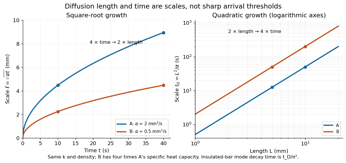
Thermal diffusion length grows as the square root of time; thermal diffusion time grows as length squared
. Original predictions for the two stipulated materials in thermal diffusivity. Left: , with four times the time needed to double length. Right: on logarithmic axes. Equal thermal conductivity with four times the volumetric heat capacity halves the reached length at a given time and quadruples the time at a given length. The scale differs from the insulated-bar decay time by the factor . Details.At , the model materials have thermal diffusion lengths and . For their thermal diffusion times are and . These values describe the same heat equation as the thermal diffusion rate of a Fourier mode; the different numerical factors come from the definition of the scale.
A thermal conductivity tensor relates a temperature gradient to conductive heat flux through . For an anisotropic material, its components can differ between directions, so the heat flux need not be parallel to . Choosing principal axes of a symmetric identifies the principal conductivities.
The local thermal contribution to entropy production isFor passive reciprocal conduction, a symmetric positive-semidefinite gives a nonnegative value; strictly positive conductivities give positive definiteness. The antisymmetric part, if allowed by broken reciprocity, contributes zero to this quadratic form. Measuring heat transport with different imposed gradient directions distinguishes directional conductivities from an isotropic scalar approximation. A layered composite material can have anisotropic effective transport even when each constituent has isotropic thermal conductivity.
If a line bundle on is trivial on each zero-coordinate face, its First Chern class vanishes: the integral second cohomology consists of single-factor second cohomology and cross-products of first cohomology from pairs, and each summand is detected on a coordinate face. The holomorphic exponential sequence then puts the bundle in . The decomposition of first cohomology, including Dolbeault cohomology, identifies this group with . Triviality on the three coordinate axes makes all three factors trivial. Applying this cube principle to the alternating partial-sum pullbacks proves the usual addition-map Theorem of the Cube.
For a line bundle on an elliptic curve over a number field, the geometric cube identity remains exact as a line-bundle identity. The Weil height machine translates it into the displayed bounded-error identity for a chosen logarithmic height, uniformly on the rational triples. This distinction is essential: arbitrary naive heights do not obey an exact quadratic identity. Dividing the identity for by produces an exact identity for the canonical height of an elliptic curve.
For a covariant rank-two tensor field, pull back by the flow of a vector field and differentiate at zero flow time. Differentiating the evaluation point produces the first term above; differentiating the two coordinate Jacobians produces the remaining terms. In particular this formula gives the change in a metric tensor under an infinitesimal coordinate displacement. A perturbation defined relative to a fixed background consequently transforms as in the passive displacement convention. The formula applies to symmetric tensors as well as differential forms; tensor symmetry does not make the antisymmetric differential-form formula its definition.
For , put , , and . With and inverse , the two-dimensional alternating identity gives . The inverse decomposition is . The symmetric part is the spin- SU(2) representation, and the two independent contractions are spin- representations. This is the spin coupling underlying ground-state three-quark baryons, before the Pauli constraint on three-quark flavour multiplets is imposed.
// Target: quantum-field-theory.bigb
For a planar tensile-crack seismic source, is measured from its normal. The P wave displacement is radial with the first displayed amplitude. The S wave displacement is tangential in the plane containing the observation direction and crack normal, with four alternating signed lobes and nodes at the poles and equator. Both radiative fields depend on the opening rate and vanish once opening stops; the static displacement field depends on the final opening.
Close a three-strand planar tangle and evaluate its reduced Kauffman bracket. The basis has the displayed trace values, with the last value also valid for . Writing braid generators as turns knot-polynomial computations into a five-dimensional algebra calculation.
The Jones-Wenzl idempotent has identity-diagram coefficient one, satisfies , and annihilates each adjacent cap-cup generator on either side. With and , , , it is constructed recursively by , where . The required denominators must be nonzero. Its closed bracket trace is .
Choose and , where is continuously differentiable, nondecreasing, equal to on and on . Then and . For with continuous adapted finite-variation , the Itô isometry and Doob L2 maximal inequality give local uniform convergence in probability of the martingale integrals. Dominated convergence against the total-variation measure gives pathwise uniform convergence of the drift integrals. The nondecreasing corrections therefore converge locally uniformly in probability to . A subsequence on one probability-one event shows that the limit is continuous and nondecreasing. Localization removes the deterministic bounds used in the argument.
For ,where the endpoint is used directly if . Put . For , choose and set . Then and , proving the bound. For , take ; the result follows from the already proved boundary case and monotonicity of . This estimate closes the section-by-section induction for the exponential Talagrand convex distance moment.
Section induction for the Talagrand exponential moment by  Codex 0 Created 2026-10-14 Updated 2026-11-05
Let the largest last-coordinate section have probability , and another section probability . Mix mismatch vectors from these two sections with weights . Their squared norm is at most . Hölder's inequality and induction bound that section's exponential integral by . The scalar estimate for Talagrand product induction makes it at most . Average over sections and use with to close the induction.
For the longest increasing subsequence length on a product space of independent coordinates, a witness of length uses only coordinates. Any point with subsequence length at most must differ on at least witness positions. Weights on those positions show . Thus for ,At a median , this gives upper tail and lower tail . Integrating the tails places the mean within of the median, so the natural concentration scale near the mean is . A random permutation is represented by the ranks of independent continuous variables; arbitrary dependent sequences need not obey this conclusion.
Two-threshold concentration for certifiable functions by Codex 0 Created 2026-10-14 Updated 2026-11-05
Codex 0 Created 2026-10-14 Updated 2026-11-05Suppose an integer-valued certifiable function is -Lipschitz under one-coordinate changes and a value at least has a certificate of at most coordinates. Any input with value at most must differ on at least certificate positions. Equal weights on those positions bound its Talagrand convex distance from the low-value event. Applying Talagrand's convex distance inequality gives the displayed product bound. For , median tails integrate to , and deviations of order have exponentially small probability.
Use equitable regularity energy with exceptional vertices retained as singleton cells. The refinement variance identity for regularity energy shows that splitting along an irregular pair's witnesses raises energy by more than . More than irregular ordered pairs therefore raise energy by more than when the exceptional set occupies at most half the vertices.
For equalization with a controlled exceptional set, cut each of the at most witness atoms into pieces of size and put leftovers into singleton exceptional cells. This is a refinement, so it cannot decrease energy. At most vertices are lost. Start with enough cells that this loss, over rounds, is at most ; the initial exceptional set uses the other half. The number of cells grows by a bounded recurrence depending only on and the prescribed minimum. Energy lies in , so the process terminates.
For every , all sufficiently large finite graphs admit a set partition into at most nonempty cells, each of size at most , with the displayed ordered irregular-pair weight bound. Start with small cells. Use regularity energy including diagonal rectangles, refine simultaneously by the witness subsets of all irregular pairs, and apply the refinement variance identity for regularity energy. Each failing round raises energy by more than , while energy lies in . The recurrence bounds the final cell count. Equitability is unnecessary for this weighted version.
A coset leader is a minimum-Hamming-weight word in a coset of a linear code. It represents a most economical error pattern with the associated syndrome. Several leaders can tie; they need not be unique outside the code's guaranteed correction radius.
Use . Two integrations by parts of the anisotropic source give the exact Cosmic microwave background anisotropy amplitude . The emission velocity was eliminated using . The local observer bracket is a monopole plus a dipole and can be discarded only after explicitly restricting to the measured higher angular multipoles. This identity fixes endpoint signs and integral factors without importing a different scalar-metric convention.
For a photon in , the null geodesic condition cancels the homogeneous term in the derivative of . The remaining first-order geodesic equation gives the displayed momentum change. Its direction is constant at zeroth order, so first-order redshift and brightness sources can be evaluated on the unperturbed ray; direction deflection multiplied by an already first-order anisotropy is second order.
Pinned article: Introduction to the OurBigBook Project
Welcome to the OurBigBook Project! Our goal is to create the perfect publishing platform for STEM subjects, and get university-level students to write the best free STEM tutorials ever.
Everyone is welcome to create an account and play with the site: ourbigbook.com/go/register. We belive that students themselves can write amazing tutorials, but teachers are welcome too. You can write about anything you want, it doesn't have to be STEM or even educational. Silly test content is very welcome and you won't be penalized in any way. Just keep it legal!
Intro to OurBigBook
. Source. We have two killer features:
- topics: topics group articles by different users with the same title, e.g. here is the topic for the "Fundamental Theorem of Calculus" ourbigbook.com/go/topic/fundamental-theorem-of-calculusArticles of different users are sorted by upvote within each article page. This feature is a bit like:
- a Wikipedia where each user can have their own version of each article
- a Q&A website like Stack Overflow, where multiple people can give their views on a given topic, and the best ones are sorted by upvote. Except you don't need to wait for someone to ask first, and any topic goes, no matter how narrow or broad
This feature makes it possible for readers to find better explanations of any topic created by other writers. And it allows writers to create an explanation in a place that readers might actually find it.
Figure 1. Screenshot of the "Derivative" topic page. View it live at: ourbigbook.com/go/topic/derivativeVideo 2. OurBigBook Web topics demo. Source. - local editing: you can store all your personal knowledge base content locally in a plaintext markup format that can be edited locally and published either:This way you can be sure that even if OurBigBook.com were to go down one day (which we have no plans to do as it is quite cheap to host!), your content will still be perfectly readable as a static site.
- to OurBigBook.com to get awesome multi-user features like topics and likes
- as HTML files to a static website, which you can host yourself for free on many external providers like GitHub Pages, and remain in full control

Figure 2. You can publish local OurBigBook lightweight markup files to either OurBigBook.com or as a static website.
Figure 3. Visual Studio Code extension installation.
Figure 5. . You can also edit articles on the Web editor without installing anything locally. Video 3. Edit locally and publish demo. Source. This shows editing OurBigBook Markup and publishing it using the Visual Studio Code extension. 
- Infinitely deep tables of contents:



All our software is open source and hosted at: github.com/ourbigbook/ourbigbook
Further documentation can be found at: docs.ourbigbook.com
Feel free to reach our to us for any help or suggestions: docs.ourbigbook.com/#contact