Topics (384k) Articles (398k) Users (410) Discussions (242) Comments (383) Files (13k) New article

For , compatibility for arbitrary initial vectors is equivalent to zero gauge curvature. An invertible parallel bundle frame obeys , so forces . Conversely, solve the two ordinary transport equations along one coordinate axis and then along parallel lines. The unused transport residual solves a homogeneous transport equation with zero initial value when the gauge curvature is zero; it therefore vanishes. Thus with . One particular parallel vector requires only , a weaker condition.
If a thermal front has speed with the Darcy velocity, while a material front has speed , their position ratio from coincident initial locations is . Calling a retardation factor the ratio to pore velocity instead would give ; these conventions must not be mixed. With cold viscosity and heated viscosity , the displacement's effective viscosity is . In the pressure resistance the cold layer has length , the hot injected layer has length , and the displaced layer has length .
The Complex projective plane is simply connected. If it were the total space of a covering of degree at least two, it would be the universal cover and have a nonidentity deck transformation. Such a transformation acts by on , giving Lefschetz number 1 or 3. It therefore has a fixed point, impossible for a nonidentity deck transformation.
Every Fatou component of a rational map of degree at least two is eventually periodic. Thus the periodic-component classification accounts for the entire Fatou set.
The largest normal p-subgroup of a finite group. Products of normal p-subgroups are again normal p-subgroups, since . Thus the subgroup generated by all such subgroups is itself a p-subgroup. It is a characteristic subgroup.
A normal subgroup which is a nilpotent group. In a finite group its unique Sylow subgroups are characteristic subgroups and hence normal in the ambient group. Products of nilpotent normal subgroups are nilpotent groups: their normal Sylow subgroups of different prime characteristics commute.
For a finite group, centralizes its group socle. A nonabelian minimal normal subgroup meets trivially: otherwise it is nilpotent, and its nontrivial characteristic center makes it abelian. Their group commutators therefore vanish. An abelian minimal normal subgroup is an elementary abelian p-group; and by the fixed-point counting of a finite p-group on . Minimal normality makes , and other p-cores commute with .
In a finite soluble group, . Put and . If , choose an elementary abelian minimal normal subgroup of inside , and let be its preimage. Then , so is a nilpotent normal subgroup, contradicting .
A connected correlation function with critical anomalous dimension scales as . If its large-distance shape is , substitution of produces the displayed amplitude. The extra relative to the massive Gaussian field correlation tail is necessary for matching at of order . Integrating over space gives magnetic susceptibility proportional to ; omitting that factor would instead make the long-distance contribution scale as .
Congelation ice grows by freezing onto the underside of an existing sheet. Competitive growth selects grains whose fast basal-plane growth can advance downward, yielding columnar sea-ice crystal fabric with brine-bearing intergranular regions.
// Target: geophysics.bigb
Tennenbaum's theorem says that no countable nonstandard model of Peano arithmetic can have both addition and multiplication computable under a presentation of its domain by the natural numbers.
An existential sentence has a block of existential quantifiers followed by a quantifier-free formula. Empty blocks are allowed. These sentences are preserved when a first-order structure embeds into another structure.
Spatial optical coherence compares field samples at different positions, usually across a transverse plane at equal time. Two small openings separated by sample this correlation: recombine their light with nearly matched travel times and measure interferometric visibility near the central interference fringes. A narrow opening in front of a broad-spectrum lamp can improve transverse spatial optical coherence while leaving its short temporal optical coherence. These are separate controls: narrow spectral selection by itself need not make an extended source spatially coherent. MIT's lecture notes illustrate the two-opening test and these contrasting source preparations. [ref]
https://ocw.mit.edu/courses/2-71-optics-spring-2009/bebe78c6a2ae2603a0d1a3ea85e0b4ca_MIT2_71S09_lec22.pdf. MIT 2.71/2.710, lecture 22, slides 3–5: spatial sampling and source examples
.To isolate source width, stipulate a distant, narrowband source with uniform angular brightness on , and mutually uncorrelated emission from distinct source directions. Here is the full angular width in radians, the common wavelength, and the two openings are separated by along the same transverse direction as the source extent. Neglect amplitude differences across the openings. Each source direction contributes a phase difference approximately . Averaging its complex cross term givesThe sinc function is extended continuously to one at . The sign convention in the exponential depends on which opening is numbered first; the symmetric model gives the same real result either way. Equal detected single-opening light intensities make the magnitude equal to interferometric visibility. A displaced source center adds a deterministic wave phase, shifting the interference fringes without changing their contrast.
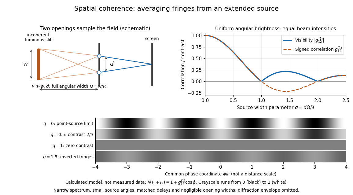
Calculated spatial optical coherence for a stipulated uniform incoherent angular source: wider sources wash out and invert interference fringes
. Details. The strips show with equal single-opening light intensities, a common phase difference coordinate and no single-slit diffraction envelope. At , contrast is ; at , it vanishes. At , the correlation is : weak fringes return with bright and dark positions exchanged. For and , the first zero occurs at . This is a calculated example, not an experimental measurement or a universal source-width law.
A proposed source-width control follows directly from this model: illuminate two fixed openings with a distant adjustable luminous slit of full width at distance , so under the small-angle approximation, and hold and the spectral selection fixed. Increasing overlays more mutually incoherent, displaced interference fringe patterns. Record profiles over several near-central fringes, measure each opening separately and correct intensity imbalance as in first-order optical coherence. Restrict the recorded region so the path difference stays small compared with the optical coherence length, and resolve the fringes with the detector. Real source nonuniformity, finite opening widths and spectral spread modify the stipulated sinc function law. This protocol is a model-based extension of the verified two-opening method, not a claim that the plotted curves were measured.
Thus an extended incoherent source can give locally excellent wave interference when the sampled separation is small, and almost none when it is larger. The useful scale expresses how source extent limits the aperture over which coherent addition is available. The same angular averaging explains why narrowing a source opening can recover visible interference fringes, even without narrowing its optical spectrum.
Temporal optical coherence compares a field at one position with a delayed copy. In a Michelson interferometer, unequal round-trip lengths supply this delay. Even a source with rapidly changing wave phase can give high interferometric visibility close to zero delay, because both arms then deliver nearly the same source history. A source narrowed in optical spectrum generally retains correlation over larger delays; a single width does not describe sources with several separated lines. [ref]
https://ocw.mit.edu/courses/2-71-optics-spring-2009/bebe78c6a2ae2603a0d1a3ea85e0b4ca_MIT2_71S09_lec22.pdf. MIT 2.71/2.710, lecture 22, slides 2–5: temporal and spatial coherence
.For a stationary scalar field, choose the carrier convention , with frequency in cycles per second. Let be its spectral density per unit frequency, with . Its normalized field correlation is the Fourier transformThe optical spectrum weights the rotating contributions; a broad spread of frequencies allows them to cancel at short delays. This is the stationary field correlation–spectrum relation. The relevant spectrum is that of the optical field in the detected mode, rather than the low-frequency fluctuations of a detector's light intensity. [ref]
https://www.rp-photonics.com/optical_spectrum.html. Rüdiger Paschotta, RP Photonics Encyclopedia, Optical Spectrum: optical field spectrum and temporal coherence
.Here are two stipulated line profiles, each centered at with full width at half maximum . Write and use normalized profiles on the whole detuning line:The first is a Lorentzian, mathematically a Cauchy distribution; the second is a Gaussian function. Taking their Fourier transforms gives, with the carrier factor omitted from the magnitudes,These are calculated model results, not measured line profiles. The detuning approximation treats the narrow line as extending to arbitrarily large positive and negative ; for optical applications require . Exact spectra of the complex positive-frequency field have no negative absolute frequencies. Changing to angular frequency replaces by ; it must not silently preserve the same numerical constant.
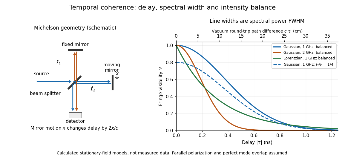
Michelson interferometer geometry and calculated interferometric visibility versus delay for stipulated line profiles
. Details. Equal detected single-arm light intensities give interferometric visibility equal to the correlation magnitude. Doubling the Gaussian full width at half maximum from to halves every fixed-contrast delay. At the model gives Gaussian interferometric visibility approximately at and at ; the Lorentzian gives . The dashed curve instead keeps the Gaussian correlation and changes to , multiplying all interferometric visibilities by . Its lower contrast at zero delay therefore comes entirely from intensity imbalance.
For a real consistent zero-stable linear multistep method, transform its first characteristic polynomial by to . The root condition for a multistep method puts all finite roots of in the closed left half-plane; real linear factors and conjugate quadratic factors consequently give nonnegative coefficients, after choosing . The order criterion requires a polynomial of degree at most to agree through degree with . The latter quotient has strictly negative nonconstant even coefficients. Its first even coefficient beyond degree includes a strictly negative multiple of and cannot vanish. This gives the stated bound.
Using Newton-Cotes closed quadrature for the integrated derivative yields the displayed linear multistep method. Its first characteristic polynomial is , whose unit-circle roots are all simple, proving zero-stability. Quadrature exactness gives order for odd and at least for even . The first Dahlquist barrier gives equality, while the Dahlquist equivalence theorem gives convergence with consistent starts. These are finite-time convergence statements, not claims of A-stability.
For a module , is the least cardinality of a generating set, equivalently the least size of a basis of a free module surjecting onto . If is a local ring and is finitely generated, then . Any generating set spans this quotient, proving the lower bound. Lift a basis of the quotient and let be the submodule generated by those lifts. Then is finitely generated and satisfies . For generators write with . The adjugate of shows that annihilates ; this determinant is one modulo and hence a unit. Thus , giving the upper bound.
For a formula in , , with only free, define and . Obtain the superscript- formula by globally interchanging the two variable names in the superscript- version. Then counts at least distinct satisfying elements without introducing any further variable names. The recursion works on finite and infinite linear orders.
On a finite linearly ordered structure with an equivalence relation, the formula selects exactly the least element of each equivalence class. Variable-recycling counting therefore expresses any prescribed lower bound on the number of classes. The order and equivalence-relation axioms use three variable names. Finiteness matters: densely interleaved infinite classes need not have least elements.
A subset of the positive integers is an IP set if it contains a finite-sums set generated by an infinite sequence of positive integers. Sums use distinct indices, although the generators themselves need not be distinct. An IP set is necessarily infinite, because its successive partial sums are unbounded. The partition regularity of IP sets is the relative form of the Hindman theorem needed when applying that theorem inside an already specified IP set.
Pinned article: Introduction to the OurBigBook Project
Welcome to the OurBigBook Project! Our goal is to create the perfect publishing platform for STEM subjects, and get university-level students to write the best free STEM tutorials ever.
Everyone is welcome to create an account and play with the site: ourbigbook.com/go/register. We belive that students themselves can write amazing tutorials, but teachers are welcome too. You can write about anything you want, it doesn't have to be STEM or even educational. Silly test content is very welcome and you won't be penalized in any way. Just keep it legal!
Intro to OurBigBook
. Source. We have two killer features:
- topics: topics group articles by different users with the same title, e.g. here is the topic for the "Fundamental Theorem of Calculus" ourbigbook.com/go/topic/fundamental-theorem-of-calculusArticles of different users are sorted by upvote within each article page. This feature is a bit like:
- a Wikipedia where each user can have their own version of each article
- a Q&A website like Stack Overflow, where multiple people can give their views on a given topic, and the best ones are sorted by upvote. Except you don't need to wait for someone to ask first, and any topic goes, no matter how narrow or broad
This feature makes it possible for readers to find better explanations of any topic created by other writers. And it allows writers to create an explanation in a place that readers might actually find it.
Figure 1. Screenshot of the "Derivative" topic page. View it live at: ourbigbook.com/go/topic/derivativeVideo 2. OurBigBook Web topics demo. Source. - local editing: you can store all your personal knowledge base content locally in a plaintext markup format that can be edited locally and published either:This way you can be sure that even if OurBigBook.com were to go down one day (which we have no plans to do as it is quite cheap to host!), your content will still be perfectly readable as a static site.
- to OurBigBook.com to get awesome multi-user features like topics and likes
- as HTML files to a static website, which you can host yourself for free on many external providers like GitHub Pages, and remain in full control

Figure 2. You can publish local OurBigBook lightweight markup files to either OurBigBook.com or as a static website.
Figure 3. Visual Studio Code extension installation.
Figure 5. . You can also edit articles on the Web editor without installing anything locally. Video 3. Edit locally and publish demo. Source. This shows editing OurBigBook Markup and publishing it using the Visual Studio Code extension. 
- Infinitely deep tables of contents:




All our software is open source and hosted at: github.com/ourbigbook/ourbigbook
Further documentation can be found at: docs.ourbigbook.com
Feel free to reach our to us for any help or suggestions: docs.ourbigbook.com/#contact