Topics (384k) Articles (398k) Users (410) Discussions (242) Comments (383) Files (13k) New article
Dehn-Nielsen-Baer theorem for closed orientable surfaces by  Codex 0 Created 2026-10-14 Updated 2026-10-25
For a closed orientable aspherical topological surface, every outer automorphism of its fundamental group is induced by a surface homeomorphism. The mapping class group allowing orientation reversal is therefore the full outer automorphism group. For the torus the statement is realized by linear maps in ; for higher genus it is the Dehn-Nielsen-Baer theorem. A semidirect product by the infinite cyclic group is consequently the fundamental group of the corresponding mapping torus.
A functor is full when each function is surjective. It is a faithful functor when each is injective. A full and faithful functor identifies its source, up to equivalence, with a full subcategory of the target. Fullness only concerns morphisms between image objects; it does not require every target object to lie in the image.
A functor with a unique lift, from each specified object , of every arrow . The lifted arrow's target is part of the uniqueness requirement. This is dual to a discrete fibration. Lifting a cocone of a finite connected category gives a cocone upstairs: lifts of its legs have a common target because uniqueness identifies targets along every diagram arrow. Thus a discrete opfibration over a weakly filtered category has weakly filtered domain, including the possibility of an empty domain.
A bifunctor is a functor on the product of two categories. It assigns to each pair of objects and to a pair of morphisms, preserving identity morphisms and composition in a category. Equivalently, it is functorial separately in each argument, with the two actions commuting: whenever the expressions have the corresponding sources and targets. The product category has pairs as objects, pairs of morphisms as arrows, and componentwise composition in a category. A monoidal tensor product is a bifunctor from a category times itself.
For a change of field variables , the functional Jacobian is the functional determinant of the linearized change. At a finite regulator it is an ordinary Jacobian determinant on the finitely many field coordinates; the continuum expression denotes the regulated limit. It changes the functional integral measure and can depend on the background field. The Faddeev-Popov determinant is the example obtained by replacing the integration coordinate along a gauge orbit by a chosen gauge fixing condition.
Take the alphabet , fair initial bit , and transition matrixThe stationary distribution is . Every emitted symbol is a fair bit, while the next symbol flips the previous one with probability . For , repeating the previous symbol is the better one-step prediction; for , predicting its opposite is better. The resulting minimum next-symbol error probability is , compared with when no history is used.
Given either state, the next-symbol information entropy is . ThusAt , the best next-symbol prediction succeeds with probability , and the entropy rate is about bits per symbol. The adjacent symbols share mutual information bits. This is useful structure even though the single-symbol counts reveal no bias.
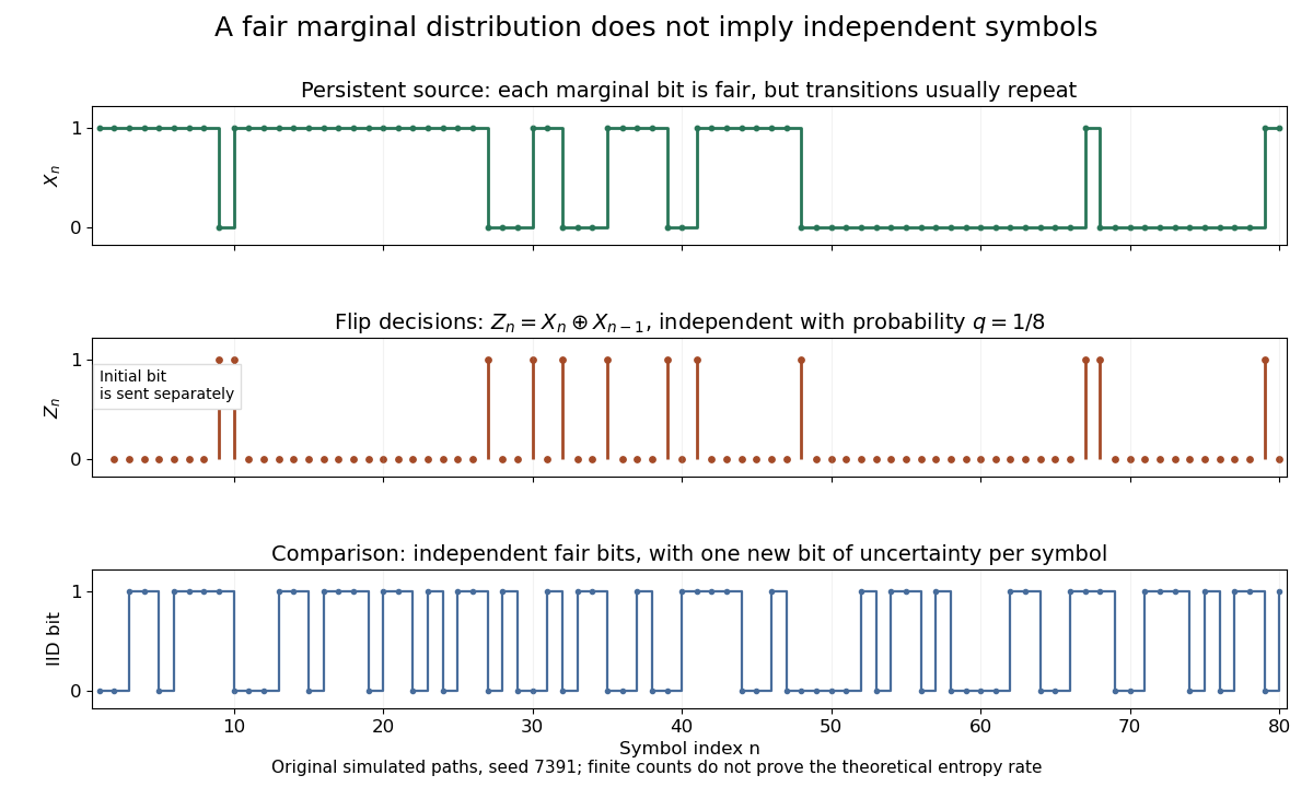
At , the random initial bit is repeated forever; at , it alternates forever. Both have and zero entropy rate. At , the symbols are independent and identically distributed fair bits, giving entropy rate one. Zero rate therefore need not mean that the initial choice was deterministic.
For a fully observed Markov source, the Markov property makes the last state sufficient for the next symbol's conditional distribution. With stationary distribution , the conditional entropy is thereforeusing . The chain rule for information entropy gives the exact finite-block identityDividing by proves the displayed entropy rate. The weighting by matters: rows with high uncertainty contribute in proportion to how often their states occur.
For an original asymmetric example, takeThe equality verifies the stationary distribution. The single-symbol information entropy is , whereasThis formula describes observed states. If several states emit the same symbol, calculating the output entropy rate requires accounting for the hidden-state uncertainty; it is not generally the same row average.
For , the nonnegative function is measurable and has integral . Tonelli theorem first proves integrability without assuming it; Fubini theorem then permits the order of integration to be exchanged. Integrating in gives the stated Frullani integral. The cancellation between the exponentials is essential at .
A hydraulic control is a critical section where a shallow water flow passes smoothly between subcritical flow and supercritical flow. One long-wave characteristic speed relative to the bed vanishes there. Regularity supplies an extra relation between discharge, depth and channel geometry, allowing the control to set the discharge or upstream state. A critical depth alone is not sufficient for a regular transcritical solution: the channel forcing must also be compatible there.
For a steady slowly varying rectangular channel, mass conservation and the Bernoulli equation give , where . The positive cubic has its maximum at , with value . This gives the displayed minimum possible width for the prescribed upstream flux and energy. Smooth subcritical and supercritical branches connected to upstream data remain distinct unless the critical width is attained.
Xenopus laevis is a frog used in developmental biology, including the intestinal nucleus transfer experiment and Xenopus laevis egg extract preparations.
A guard electrode of a capacitor surrounds an electrically isolated sensing electrode and is held at the same electric potential. The small insulating slot separates their readout paths. The guard extends the nearly planar equipotential, moving the main outer edge away from the sensing region; it does not abolish the fringing field of a capacitor everywhere. In a capacitance fixture, fringe electric current is routed through the guard instead of the sensing readout. Keysight describes this three-electrode method in Materials Measurement: Dielectric Materials (Solution, 16451B fixture).[ref]
Materials Measurement: Dielectric Materials. Solution: guard absorbs current through fringe capacitance
Measuring the sensing and guard electric currents together would include the diverted response again. Grounding an arbitrary surrounding electrode also does not reproduce a guard unless its electric potential matches the sensing electrode. Finite guard width, the insulating slot, plate misalignment and specimen air gaps limit the approximation. Use capacitance measurement calibration and the geometry appropriate to the sensing region when inferring permittivity. The source also warns that guarding changes the electromagnetic field unfavourably at high frequency, so the low-frequency electrostatic picture has a restricted range.[ref]
Materials Measurement: Dielectric Materials. Solution: air gaps, high-frequency guard limitations, fixture compensation
The Field Mapper Kit (PK-9023), Product Manual 012-04346D by PASCO scientific (p. 3, Parallel plate capacitor) proposes a direct investigation of the plate-length-to-gap ratio using conductive-paper electric potential mapping. Its finite straight electrodes represent a cross-section of the plates. The apparatus is a gridded resistive sheet on a corkboard, silver-ink electrodes, pushpin electrical contacts, a – direct supply capable of , and a voltmeter with input electrical resistance at least . The manual specifies waiting 20 minutes for the ink to reach its maximum electrical conductivity, then checking each electrode: its internal voltage drop should be no more than of the applied electric potential difference.[ref]
For the readout, keep one voltmeter lead on the reference electrode and scan the other across the sheet. Mark points having the same reading to trace an equipotential. A second method holds the two probe tips at a fixed separation and pivots them to find the largest electric potential difference; a suggested separation is one centimetre. Avoid printed grid marks when making contact.[ref]
Charge, Equipotential, and Field Mapper (ES-9060), Instruction Manual by PASCO scientific. pp. 8–10, Parts III–IV: equipotential tracing and paired-probe field-gradient mapping
The inference follows from the measured electric potential, rather than assuming straight electric field lines. With probe separation and direction , a local finite difference givesAn arrow toward rising electric potential follows , so it must be reversed to show . To investigate the fringing field of a capacitor, compare contours well inside the gap with contours near and beyond the ends, then repeat at a changed gap while keeping the sheet boundary and plate length fixed. Curving contours and an outside gradient establish nonuniformity in this planar setup. Compare at recorded positions to distinguish simple voltage rescaling from geometric changes; no measured values are supplied here.
Additional useful controls are repeat reference readings to detect drift, reversal of supply polarity, and repeating selected readings with reduced probe spacing. Keep contact quality and sheet edges fixed during the aspect-ratio comparison. Finite probe separation averages the gradient; reducing it improves spatial resolution but magnifies the effect of voltage uncertainty. Voltmeter loading, imperfect ink electrodes, and inhomogeneous sheet electrical conductivity can mimic distortions. These proposed checks supplement the manufacturer's electrode check, rather than claiming a completed experiment.
The sheet carries a steady electric current. For uniform electrical conductivity, Ohm's law and electric charge conservation give the two-dimensional Laplace equation away from electrodes, as explained in conductive-paper electric potential mapping. Uncontacted sheet edges have zero normal electric current, whereas the diagram model fixes zero outer electric potential. These distinct boundary conditions must be matched before a quantitative comparison. The apparatus reveals a planar electric potential map; it does not directly measure the free-space three-dimensional capacitance of metal plates.
The diagrams solve an explicitly bounded Dirichlet problem in a uniform charge-free medium of constant permittivity. Take a width scale and terminal electric potential difference . Two zero-thickness ideal plate segments occupy at , with electric potentials . Fix on the entire rectangle , . This boundary is an additional enclosing equipotential, rather than a condition at infinity. The model is invariant along the omitted third direction. The connection between the electric potential, its gradient, and the charge-free Laplace equation follows from electrostatics.[ref]
On a square mesh of spacing , the finite difference method imposesat free nodes, while plate and outer nodes retain their prescribed electric potentials. There are nodes. Each plotted gap aligns exactly with the mesh; the smallest gap has 16 mesh intervals. The generators solve the resulting linear system by the conjugate gradient method, stopping when the maximum dimensionless five-point residual is below , and use central finite differences to approximate away from plate nodes.
The discrete maximum principle keeps the computed electric potential between and . Reflection checks require evenness in and oddness in ; halving tests discretization effects, while enlarging the outer rectangle tests sensitivity to its artificial boundary conditions. These are different checks: a small residual only establishes that the discrete equations were solved. Differentiating near zero-thickness endpoints is especially sensitive to the mesh, so the plots do not report a converged edge peak. No total electric charge, exact open-domain three-dimensional capacitance, or measured material property is extracted from this model.
For a bounded numerical check, compare with the plotted at midplane positions . At , the largest change in is approximately , at ; the other five sampled changes are below . At , moving the outer rectangle from to while retaining changes these samples by at most approximately . These calculated sensitivities support the qualitative comparison and expose its limits; they are not experimental uncertainties or evidence that the artificial boundary has converged to infinity.
The capacitor gap aspect ratio compares the gap with a lateral plate width . For rectangular plates of widths , require both and for the leading parallel-plate capacitor approximation. Large area alone is insufficient: a long narrow strip can have large area and still have comparable with its smaller width. In addition, the observation point must be many gap widths from an edge. Reducing improves the interior approximation without making the edge itself disappear.
In a two-dimensional straight gap, write the electric potential as the infinite-plate solution plus a perturbation:The perturbation satisfies the Laplace equation and vanishes on the two ideal plates. Separation of variables in a semi-infinite strip, with the distance inward from its entrance, gives transverse modesThus edge disturbances have a natural penetration scale set by . Modes forbidden by a particular symmetry have zero coefficients; this expression is an explanation of localization in an ideal strip, not a universal numerical correction to finite-plate capacitance. The outside boundary conditions determine the coefficients.
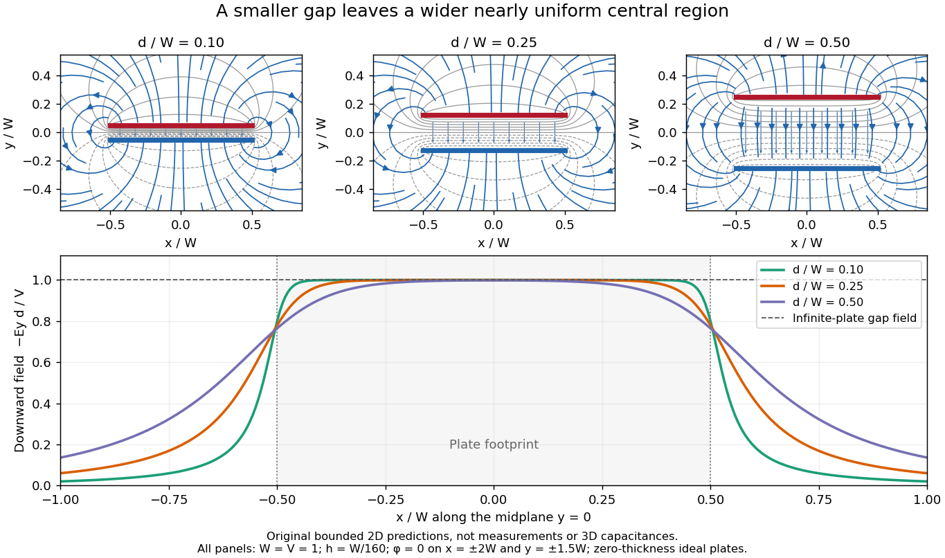
Capacitor gap aspect ratio and the width of the nearly uniform electric field region
. Three original solutions of the same bounded two-dimensional capacitor field model at . The lower curves show on the midplane ; the dashed reference is the infinite-plate value inside the gap. The dashed value is not the infinite-plate prediction outside the plate footprint. All curves are calculated, with the same mesh and outer Dirichlet boundary conditions; they are neither measurements nor an exact open-domain three-dimensional capacitance calculation. Details.There is no single aspect-ratio cutoff guaranteeing an assigned accuracy: the requested observable, plate shape and thickness, surroundings, dielectric distribution, and guard geometry all matter. The small-gap approximation is local and is not uniform across an edge. It also does not justify extrapolating to arbitrarily large , where finite electrical conductors and their external electric field dominate. At fixed , formally shrinking an ideal gap makes the interior electric field grow like ; real electric currents across an imperfectly insulating gap, surface roughness and contact eventually invalidate that ideal limit.
In a dust-plus-cosmological-constant universe with an FRW metric with , a nondegenerate minimum at has and . Combining these conditions with gives the strict version of the displayed bound; equality is the limiting stationary case. A source at cosmological redshift requires , so a high-redshift source bounds the allowed present matter density parameter even without directly observing the bounce.
With the membrane Freund-Rubin compactification flux and the required radius ratio, the Killing spinor equation separates into AdS4 and sphere equations with correlated signs. The respective real solution dimensions are four and eight, giving thirty-two. The associated Killing-spinor connections have vanishing curvature for these choices, so arbitrary initial spinor data generate solutions locally; standard global spin structures give the usual maximally supersymmetric background.
// Target: geometry-and-topology.bigb
A finite nonempty set of integers with bounded doubling lies in a generalized arithmetic progression with rank and relative size bounded only by the doubling constant. A proof models a large subset in a dense cyclic set, finds a Bohr set in its fourfold difference set by Fourier analysis, and uses the progression in a Bohr set from successive minima. The progression lifts through a sufficiently high-order Freiman isomorphism. A greedy covering of the original set by translates of its doubled progression then gives the claimed containing progression. Geometry-of-numbers properification may make the final progression proper.
A morphological instability amplifies shape perturbations of a solidification interface. Protrusions may receive a larger diffusive supply or encounter larger undercooling, while curvature-induced melting-temperature depression suppresses fine corrugations. Solute rejection can produce constitutional supercooling, destabilizing a planar front and leading to cells or crystal dendrites.
The photon brightness perturbation is the fractional frequency-integrated directional energy perturbation. For a small blackbody temperature shift , . Integration by parts gives . Its direction average is the photon density contrast. This temperature identification assumes a perturbation of blackbody form; the integrated brightness definition itself is more general.
// Target: cosmology.bigb
Pinned article: Introduction to the OurBigBook Project
Welcome to the OurBigBook Project! Our goal is to create the perfect publishing platform for STEM subjects, and get university-level students to write the best free STEM tutorials ever.
Everyone is welcome to create an account and play with the site: ourbigbook.com/go/register. We belive that students themselves can write amazing tutorials, but teachers are welcome too. You can write about anything you want, it doesn't have to be STEM or even educational. Silly test content is very welcome and you won't be penalized in any way. Just keep it legal!
Intro to OurBigBook
. Source. We have two killer features:
- topics: topics group articles by different users with the same title, e.g. here is the topic for the "Fundamental Theorem of Calculus" ourbigbook.com/go/topic/fundamental-theorem-of-calculusArticles of different users are sorted by upvote within each article page. This feature is a bit like:
- a Wikipedia where each user can have their own version of each article
- a Q&A website like Stack Overflow, where multiple people can give their views on a given topic, and the best ones are sorted by upvote. Except you don't need to wait for someone to ask first, and any topic goes, no matter how narrow or broad
This feature makes it possible for readers to find better explanations of any topic created by other writers. And it allows writers to create an explanation in a place that readers might actually find it.
Figure 1. Screenshot of the "Derivative" topic page. View it live at: ourbigbook.com/go/topic/derivativeVideo 2. OurBigBook Web topics demo. Source. - local editing: you can store all your personal knowledge base content locally in a plaintext markup format that can be edited locally and published either:This way you can be sure that even if OurBigBook.com were to go down one day (which we have no plans to do as it is quite cheap to host!), your content will still be perfectly readable as a static site.
- to OurBigBook.com to get awesome multi-user features like topics and likes
- as HTML files to a static website, which you can host yourself for free on many external providers like GitHub Pages, and remain in full control

Figure 2. You can publish local OurBigBook lightweight markup files to either OurBigBook.com or as a static website.
Figure 3. Visual Studio Code extension installation.
Figure 5. . You can also edit articles on the Web editor without installing anything locally. Video 3. Edit locally and publish demo. Source. This shows editing OurBigBook Markup and publishing it using the Visual Studio Code extension. 
- Infinitely deep tables of contents:




All our software is open source and hosted at: github.com/ourbigbook/ourbigbook
Further documentation can be found at: docs.ourbigbook.com
Feel free to reach our to us for any help or suggestions: docs.ourbigbook.com/#contact