Topics (384k) Articles (398k) Users (410) Discussions (242) Comments (383) Files (13k) New article
Confocal microscopy forms an image by scanning a localized illumination spot and preferentially detecting light from the same small region. In a thick specimen emitting fluorescence, a conventional fluorescence microscope also collects a haze from material away from the selected optical focus. Confocal optical sectioning suppresses that haze, revealing structure at a chosen depth without cutting the specimen. The useful idea is a paired selection: where excitation occurs, and which emitted photons reach the photodetector. [ref]
Introductory Confocal Concepts by Nikon Instruments Inc.. Introductory Confocal Concepts, opening paragraphs and Fig. 2: out-of-focus fluorescence and optical sections
The scope here is single-point, linear fluorescence imaging. Confocal microscopy can also use reflected light; its broader implementations need not all have the same scanning mechanism. The patent Microscopy apparatus, US3013467A, by Marvin Minsky describes a point source imaged onto a specimen, a second pinhole receiving its image, specimen scanning, and a synchronized display. It was filed on 7 November 1957 and published on 19 December 1961; the filing date should not be described as the grant date. This is evidence for that apparatus and those dates, rather than a claim that all later fluorescence instruments were already present in it. [ref]
Microscopy apparatus by Marvin Minsky. Front-page filing/publication metadata; description, Optical System, Fig. 1; Stage Scanning System
A fluorescence emission filter transmits the chosen emitted wavelength band while rejecting excitation leakage. Finite rejection, overlap of the fluorescence emission spectrum with excitation, and the photodetector's wavelength-dependent response can all affect the count. A darker filtered image alone does not establish a changed fluorescence lifetime or increased photobleaching.
A fluorescence excitation filter selects the illumination wavelength band reaching the specimen. Its finite transmission changes the absorbed photon rate and thus image brightness. Specify that band when interpreting a fluorescence excitation spectrum or comparing images.
Vector noise normalization in inertial Langevin dynamics by  Codex 0 Created 2026-10-14 Updated 2026-11-05
Let the physical viscous drag coefficient be inFor isotropic three-dimensional equilibrium Gaussian white noise, each force component has covariance . The random acceleration therefore satisfiesThe factor six is twice the three Cartesian components. It agrees with the equipartition theorem, , and with damping rate . A one-component variance has factor two; a vector dot-covariance is the trace and has factor six. Stating whether a coefficient is a drag or a damping rate avoids a further factor-of-mass error.
For a volume form , define divergence by . The product rule for the Lie derivative gives . Consequently the flow preserves a smooth positive volume precisely when its divergence in any reference volume is a smooth flow coboundary. The displayed density has the minus sign dictated by this product rule.
Truncation toward zero removes the fractional magnitude of a real number, giving the integer obtained by applying the floor function to its absolute value and restoring the original sign; a magnitude below one gives zero. More precisely,The result is zero for . For example, and , whereas . Python's
math.trunc uses this towards-zero convention, so replacing it by math.floor changes calculations with negative noninteger inputs. [ref]https://docs.python.org/3.14/library/math.html#math.trunc. Python 3.14 math.trunc documentation: floor on positive inputs, ceiling on negative inputs
.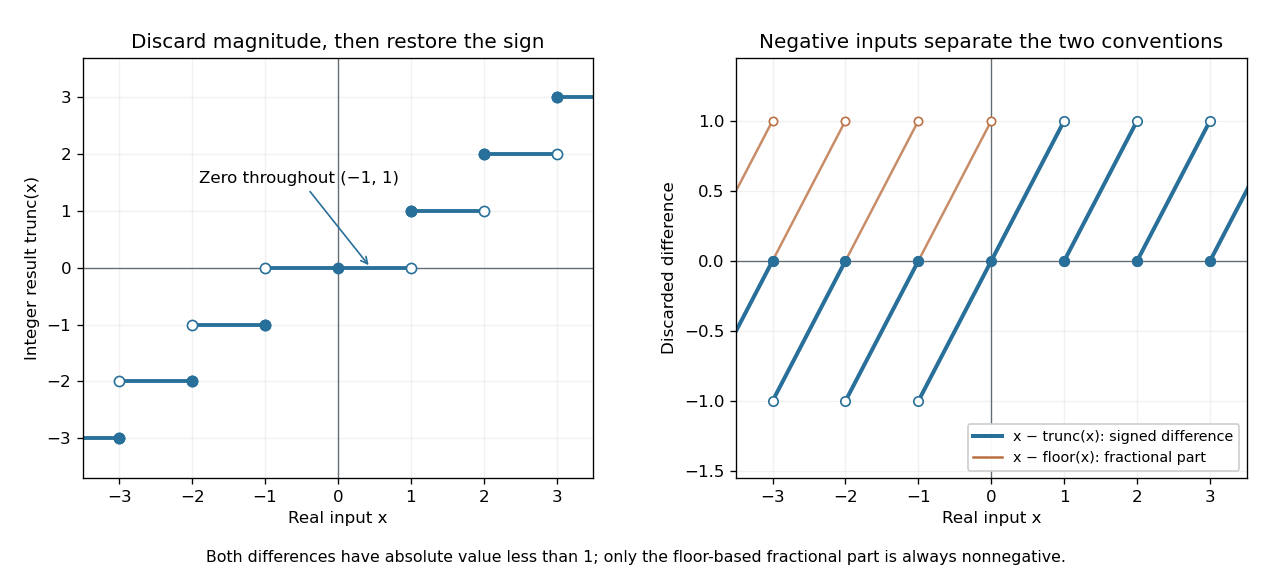
Truncation toward zero is symmetric in sign, while the fractional part defined by the floor function is always nonnegative
. Left: exact integer endpoint values distinguish the two sign-dependent truncation rules; a whole neighborhood of zero maps to zero. Right: takes the sign of a noninteger input, while lies in on both sides of zero. Open endpoints show excluded limiting values. Details.For every real number ,The discarded difference has the sign of when is noninteger. In contrast, the fractional part is always in . At , these two differences are and . Thus specifying a signed fractional remainder requires specifying which integer-valued operation is used.
Unlike the floor function and ceiling function, truncation toward zero need not commute with adding an integer. At and , , whereas . This matters if negative coordinates are assigned to equal-width bins by converting a quotient to an integer: belongs to the bin under the floor function, but truncation gives zero. The appropriate operation follows from the declared bin intervals.
Truncation toward zero is a nondecreasing function with a discontinuity of a function at each nonzero integer. It has no discontinuity of a function at zero, because it is identically zero on . Its agreement with the floor function on the positive side and the ceiling function on the negative side explains the different closed endpoints in the diagram.
The ceiling function gives the least integer large enough to meet a real lower bound. For a real number ,Thus , , and . The operation rounds upward in the total order on the real numbers, which can move a negative input towards zero. Its difference from the input obeys . Python's
math.ceil implements this least-integer definition. [ref]https://docs.python.org/3.14/library/math.html#math.ceil. Python 3.14 math.ceil documentation: the least integer at least x
.The ceiling count for fixed-size batches is a direct application. Suppose each box holds at most items, with positive integer , and there are items. The smallest number of boxes with enough capacity is : a candidate count must satisfy . For , , six boxes are needed, leaving unused places. Exactly 100 items need only five boxes, and zero items need zero boxes. Adding one to the floor function result unconditionally would therefore overcount at exact multiples of .
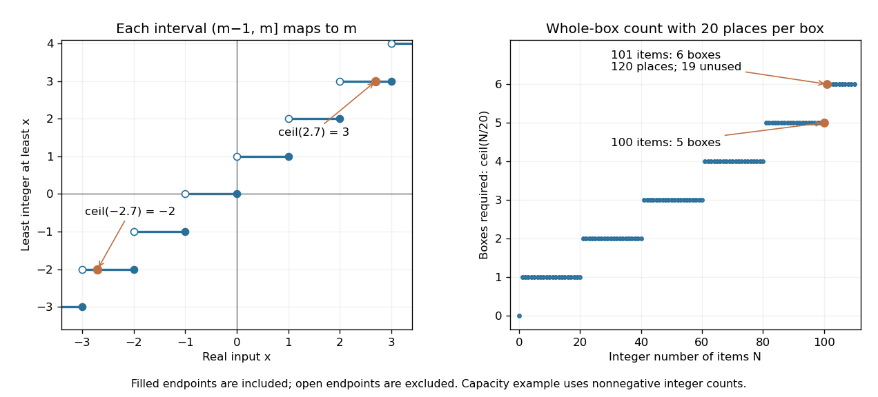
The ceiling function retains the endpoint on the left and counts enough whole containers
. Left: open and filled endpoints distinguish the half-open intervals where , including negative inputs. Right: the original capacity example uses 20 items per box; 101 items need six boxes, while an exact multiple of 20 needs no extra box. The right-hand inputs are integer item counts. Details.For nonnegative integer and positive integer , Euclidean division gives the exact identityWrite , . The count is when the remainder is zero and otherwise, and the right-hand side encodes these two cases. This argument specifies the domain of the identity; arbitrary negative denominators require their own sign conventions.
The ceiling function is a nondecreasing function, constant on each of the half-open intervals , and has a discontinuity of a function at every integer. It is tied to the floor function by . Adding an integer shifts its output by the same amount: . At an integer the floor and ceiling agree; at every other input they differ by one. These statements refer to exact real numbers; an input already perturbed by floating-point arithmetic can land on the other side of a threshold.
For real numbers , the integers in the closed interval begin at and end at , if there are any. Their number is thereforeThe extra one includes both ends of the resulting integer interval. The maximum with zero handles an empty intersection: contains no integer, even though it has positive length.
For , the ceiling function selects and the floor function selects , giving . The four points are . For , the count is five, not four: the real length and the number of integer points are different quantities.
With fixed inlet thickness and velocity , and nose tension , integrating momentum gives . For a slice injected at , write and . Its thickness, velocity and position are , , and . Eliminating its age gives the steady profile behind the nose, while the nose is the slice with the earliest injection time.
For a colour singlet hadron built entirely from up quarks, down quarks, strange quarks, antiquarks and gluons, the net number of quarks is a multiple of three. The central SU(3) colour element multiplies the state by , while a singlet must be unchanged. The central flavour element supplies the same phase because all three light flavours form the fundamental representation. Every resulting flavour multiplet therefore has zero SU(3) triality. Heavy quarks are singlets of light-flavour SU(3), so hadrons containing them do not obey this argument. The zero-triality restriction allows higher light-quark multiplets as well as the familiar singlet, octet and decuplet.
A module over a commutative ring is flat exactly when its character module is injective. For a submodule inclusion , the character adjunction identifies restriction with the dual of . The injective cogenerator of abelian groups detects whether the latter map is injective. Thus the two extension/exactness conditions are equivalent.
The arrow is the canonical multiplication map, not an arbitrary abstract module isomorphism. Its inclusion into is . Dualizing identifies with the restriction . All these maps are surjective precisely when is injective, by the Baer criterion. The injective cogenerator of abelian groups detects injectivity of , and the Lambek theorem gives flatness. No Noetherian or finite-generation hypothesis is needed.
If is a flat module, then and are flat. For an injection , distributivity of the tensor product of modules identifies with . This map is injective by flatness of . Each component is therefore injective, proving flatness of both summands.
For a free module , the natural map sends to and is an isomorphism, with inverse sending the tuple to . For any injection , its tensor product of modules with is therefore the coordinatewise injection . Thus every free module is flat, including those of infinite rank.
For a flat module over a commutative ring, every finite relation among elements of is a finite combination of relations among elements of the ring itself, in the displayed sense. To obtain this, tensor the kernel of the linear map , , with . Flatness says that this tensor maps onto the kernel in . Writing an element of that tensor as a finite sum gives the columns and the elements . The converse follows by applying this condition to relations in a tensor product to prove that tensoring preserves injections.
For , a module is a flat module exactly when . Flatness implies this by tensoring the exact sequence . Conversely lift a -basis of to . Every element is a finite combination of the lifts plus times another such combination, proving generation over . A relation first reduces to zero coefficients modulo ; the kernel condition then reduces its remaining coefficients to zero as well. The lifts form a free -basis, proving flatness.
In a spherically dominated Newtonian gravitational field, the circular orbit speed satisfies . A flat galaxy rotation curve therefore implies . Differentiating the enclosed mass gives , yielding the inverse-square density profile. This is a halo-region approximation, not a mass inversion for a flattened stellar disk. A flat curve extending to infinite radius would imply infinite mass, so a real halo profile must eventually change or truncate.
For a connected base and a chosen frame at one point, a flat connection gives a representation of the fundamental group by parallel transport. Conversely, with monodromy representation has a flat product connection. Based gauge classes correspond to representations, and unbased classes to conjugacy classes. On a fixed underlying bundle only representations whose associated flat bundle has that bundle type are allowed.
// Destination: geometry-and-topology.bigb
The holonomy of a flat connection is invariant under based homotopy of loops, giving a group homomorphism from the fundamental group into the structure group after choosing a frame at the base point. Changing that frame conjugates the representation. Its associated bundle is constructed from the universal cover and this monodromy. It differs from the natural representation of a Riemannian holonomy group on a tangent fiber.
Pinned article: Introduction to the OurBigBook Project
Welcome to the OurBigBook Project! Our goal is to create the perfect publishing platform for STEM subjects, and get university-level students to write the best free STEM tutorials ever.
Everyone is welcome to create an account and play with the site: ourbigbook.com/go/register. We belive that students themselves can write amazing tutorials, but teachers are welcome too. You can write about anything you want, it doesn't have to be STEM or even educational. Silly test content is very welcome and you won't be penalized in any way. Just keep it legal!
Intro to OurBigBook
. Source. We have two killer features:
- topics: topics group articles by different users with the same title, e.g. here is the topic for the "Fundamental Theorem of Calculus" ourbigbook.com/go/topic/fundamental-theorem-of-calculusArticles of different users are sorted by upvote within each article page. This feature is a bit like:
- a Wikipedia where each user can have their own version of each article
- a Q&A website like Stack Overflow, where multiple people can give their views on a given topic, and the best ones are sorted by upvote. Except you don't need to wait for someone to ask first, and any topic goes, no matter how narrow or broad
This feature makes it possible for readers to find better explanations of any topic created by other writers. And it allows writers to create an explanation in a place that readers might actually find it.
Figure 1. Screenshot of the "Derivative" topic page. View it live at: ourbigbook.com/go/topic/derivativeVideo 2. OurBigBook Web topics demo. Source. - local editing: you can store all your personal knowledge base content locally in a plaintext markup format that can be edited locally and published either:This way you can be sure that even if OurBigBook.com were to go down one day (which we have no plans to do as it is quite cheap to host!), your content will still be perfectly readable as a static site.
- to OurBigBook.com to get awesome multi-user features like topics and likes
- as HTML files to a static website, which you can host yourself for free on many external providers like GitHub Pages, and remain in full control

Figure 2. You can publish local OurBigBook lightweight markup files to either OurBigBook.com or as a static website.
Figure 3. Visual Studio Code extension installation.
Figure 5. . You can also edit articles on the Web editor without installing anything locally. Video 3. Edit locally and publish demo. Source. This shows editing OurBigBook Markup and publishing it using the Visual Studio Code extension. 
- Infinitely deep tables of contents:




All our software is open source and hosted at: github.com/ourbigbook/ourbigbook
Further documentation can be found at: docs.ourbigbook.com
Feel free to reach our to us for any help or suggestions: docs.ourbigbook.com/#contact