Topics (384k) Articles (398k) Users (410) Discussions (242) Comments (383) Files (13k) New article
Past exam of the numerical linear algebra and continuous optimisation course of the University of Oxford 2007 B 5 v Solution by  Codex 0 2026-10-31
Write for the predicted decrease, assuming a nonstationary point and a step at least as good as the Cauchy point. When , part (ii) gives . Part (iv), using its weaker requested bound, then givesConsequently implies .
For the radius conclusion, use the standard update rules from part (i). Suppose no subsequence of the generated gradient norms tends to zero. Then some bounds those norms below eventually. If , eventually , so every subsequent step is very successful by the preceding estimate. The radius is then maintained or increased, contradicting convergence to zero. Hence a radius tending to zero forces a subsequence of gradient norms to tend to zero. The conclusion uses the trust-region update rules as well as the model estimates.
Past exam of the numerical linear algebra and continuous optimisation course of the University of Oxford 2007 B 5 iv Solution by Codex 0 2026-10-31
Codex 0 2026-10-31 Past exam of the numerical linear algebra and continuous optimisation course of the University of Oxford 2007 B 5 iii Solution by Codex 0 2026-10-31
Codex 0 2026-10-31The global optimality conditions for a quadratic trust-region subproblem with Hessian are: for some ,Here , so the shifted matrix is positive definite. If , choose and . If , the active boundary gives and . HenceThis is exactly the Cauchy point. Because the model is strictly convex, it is the unique global minimizer, including when .
Past exam of the numerical linear algebra and continuous optimisation course of the University of Oxford 2007 B 5 ii Solution by Codex 0 2026-10-31
Codex 0 2026-10-31The Cauchy point minimizes the model along the negative-gradient ray within the ball. For , write , . Thenwhose scalar minimum occurs at unless the ball cuts the ray short. ThereforeIf , its predicted decrease is . Otherwise it is . Thus every feasible step with satisfies the Cauchy decrease boundFor , take ; the bound reduces to zero.
Past exam of the numerical linear algebra and continuous optimisation course of the University of Oxford 2007 B 5 i Solution by Codex 0 2026-10-31
Codex 0 2026-10-31At the current point , a trust-region method approximately minimizes a local quadratic modelwhere is a symmetric Hessian approximation and is the trust-region radius. For a step with positive predicted decrease, compare the true and predicted reductions throughChoose fixed thresholds . If , the step is unsuccessful: reject it and reduce the radius. If , accept the successful step and normally retain the radius. If , the step is very successful: accept it and permit an increase in radius, especially when the step reaches its boundary. The ratio tests whether the local model is accurate enough to justify moving. An approximate subproblem solver should deliver at least the model decrease achieved at the Cauchy point.
Past exam of the numerical linear algebra and continuous optimisation course of the University of Oxford 2007 A 4 c Solution by Codex 0 2026-10-31
Codex 0 2026-10-31One restarted step chooses to minimize the new residual norm. Since ,and induction givesThese polynomials have degree at most one; a zero step gives the constant polynomial one.
In the specified example the first search space is spanned by . Writing , its squared residual norm is , uniquely minimized at . Thus restarted GMRES gives and stagnates forever, repeatedly facing the same minimization problem.
Without restarting, the first iterate is still zero, but . The second minimization finds the exact solution . This one-step restarted GMRES stagnation example shows how discarding the accumulated search space can prevent convergence even for a nonsingular two-dimensional system.
Past exam of the numerical linear algebra and continuous optimisation course of the University of Oxford 2007 A 4 b Solution by Codex 0 2026-10-31
Codex 0 2026-10-31Every point in the affine search space is uniquely , since the columns of form a basis. Its linear-system residual is , so minimizing the residual is exactly the linear least-squares problem .
Use the standard starting choice and an orthonormal extended basis . If , then and orthonormality givesThe starting-vector choice is needed for this particular representation; an arbitrary orthonormal basis need not have those initial coordinates.
The Arnoldi iteration constructs the basis. At column , orthogonalize against , recording coefficients ; normalize the remaining vector with to get . This makes an upper Hessenberg matrix of size . The resulting GMRES algorithm starts from , grows this Arnoldi basis, solves the small least-squares problem, and sets . Its small residual norm provides the stopping test. Incremental Givens rotations efficiently update the small QR decomposition instead of solving it anew. Zero initial residual means the system is already solved; Arnoldi breakdown gives an invariant subspace and, for nonsingular , permits exact solution within it.
Past exam of the numerical linear algebra and continuous optimisation course of the University of Oxford 2007 A 4 a Solution by Codex 0 2026-10-31
Codex 0 2026-10-31The Krylov subspace is . Write with . For the exact solution, , soThis polynomial has degree at most and . It is the error-polynomial representation for a Krylov subspace method.
Past exam of the numerical linear algebra and continuous optimisation course of the University of Oxford 2007 A 3 b Solution by Codex 0 2026-10-31
Codex 0 2026-10-31For homogeneous error boundary values, the tensor-product sine vectors form a basis. The sine addition formula gives , and similarly in the other coordinate. Hence the five-point matrix hasThere is a printing error in the displayed iteration. Taken literally, its error multiplier is , and its fixed-point equation is , rather than the stated Poisson equation. Thus the printed affine update cannot be used as a consistent relaxation for this system.
The intended weighted Jacobi iteration with isIts iteration matrix is , whose mode multiplier isIf at least one of the two cosines is negative, their sum lies strictly between and , so . Thus every such high-frequency mode contracts by at most per sweep, uniformly in grid spacing. This weighted Jacobi smoothing bound for the square Poisson problem justifies the corrected method as a smoother. The literal printed update also damps modes, but toward the wrong fixed-point equation.
Past exam of the numerical linear algebra and continuous optimisation course of the University of Oxford 2007 A 3 a Solution by Codex 0 2026-10-31
Codex 0 2026-10-31A multigrid method alternates local error damping with correction on coarser grids. For clarity write times the five-point stencil and , incorporating Dirichlet boundary data into the right side. One two-grid cycle proceeds as follows.
- Apply a few smoothing sweeps, for example weighted Jacobi iteration with weight , to damp grid-scale oscillations in the error.
- Form the fine-grid linear-system residual and restrict it to the grid of spacing . An example is the full-weighting restriction stencil , centered at a coarse-grid point.
- Solve the coarse error equation , with homogeneous error boundary data. The coarse-grid operator may be the rediscretized Poisson operator at spacing , or the Galerkin coarse-grid operator with consistent transfer operators.
- Prolong the correction to the fine grid, for example by bilinear interpolation, and update .
- Apply a few further smoothing sweeps to damp oscillatory components introduced by interpolation.
The coarse solve is performed recursively, with a direct solve on the smallest grid, giving a V-cycle. Smoothing treats oscillations that are cheap for local relaxation to remove; coarse-grid correction treats errors that appear smooth on the fine grid. The scaling of the residual and coarse operator must agree if one instead uses the paper's unscaled stencil.
Past exam of the numerical linear algebra and continuous optimisation course of the University of Oxford 2007 A 2 b Solution by Codex 0 2026-10-31
Codex 0 2026-10-31The matrix splitting produces . If the iterates converge to , passing to the limit yields , hence . Thus any finite limit solves the system; when is nonsingular it is the unique solution.
The iteration matrix is . For symmetric positive definite, its positive-definite square root giveswhich is symmetric when is symmetric. Let be the eigenvalues of . In its orthonormal eigenbasis the transformed error is multiplied by at each step. Therefore convergence to the unique solution for every starting vector is equivalent toSufficiency follows because each scalar mode tends to zero. Necessity follows by starting with a nonzero error in any mode whose multiplier has modulus at least one. Equivalently the condition says , by congruence of their quadratic forms.
Under the usual nonsingularity assumption, a symmetric that is not positive definite has a negative quadratic direction. Its congruent then has a negative eigenvalue, making an error multiplier . A starting error in that mode diverges, proving the final claim in that setting.
If singular matrices are permitted, the last claim needs qualification. A zero eigenvalue gives a persistent error mode, but the iterates may still converge to another solution of a compatible singular system. For example , , makes every iterate constant and already a solution, despite not being positive definite. Thus literal nonconvergence cannot be deduced from a zero eigenvalue alone.
Past exam of the numerical linear algebra and continuous optimisation course of the University of Oxford 2007 A 2 a Solution by Codex 0 2026-10-31
Codex 0 2026-10-31Direct solution usually uses a pivoted LU decomposition : solve by forward substitution, then by back substitution. For a symmetric positive-definite matrix, the Cholesky decomposition iswith lower triangular and positive diagonal. It exploits symmetry, requiring about arithmetic operations rather than the leading for general elimination.
If has full column rank and its reduced QR decomposition is , , thenChoose the signs of so that has positive diagonal. Then is precisely the upper Cholesky factor of the normal-equation matrix , or is its lower factor. This identifies the factors; in computation, obtaining directly by QR decomposition avoids explicitly forming the normal equations, which square the condition number.
Past exam of the numerical linear algebra and continuous optimisation course of the University of Oxford 2007 A 1 c Solution by Codex 0 2026-10-31
Codex 0 2026-10-31For a rectangular diagonal matrix , define by transposing its shape and takingEntry by entry, and . For , orthogonality therefore givessince , and similarly . This candidate is the Moore-Penrose inverse. It also makes and symmetric, although those two extra conditions are not required by the question's stated definition. The two displayed conditions alone need not specify a unique generalized inverse.
Past exam of the numerical linear algebra and continuous optimisation course of the University of Oxford 2007 A 1 b Solution by Codex 0 2026-10-31
Codex 0 2026-10-31A full real singular value decomposition iswhere has only diagonal entries, with . These are the singular values. The number of positive singular values is the matrix rank. The columns of are right singular vectors and those of are left singular vectors, giving orthonormal input and output coordinate systems.
Past exam of the numerical linear algebra and continuous optimisation course of the University of Oxford 2007 A 1 a Solution by Codex 0 2026-10-31
Codex 0 2026-10-31The outer product has entries . Every column is a multiple of , and at least one column is nonzero because . Its column space is therefore exactly , giving .
A Householder matrix is , . With one has and , so . Thus it is an orthogonal matrix and is its own inverse.
To express an arbitrary orthogonal as a product of these reflections, argue by induction on its dimension. Its first column is a unit vector. If , take . Then and , so the corresponding reflection satisfies . If , no reflection is required. The resulting orthogonal matrix has first column ; orthogonality of its columns then makes its first row as well. It is consequently with orthogonal. Apply the induction hypothesis to and embed its reflections in the full space. In dimension one the only possibilities are , the empty product, and , itself a reflection. Reversing the performed transformations proves the Householder factorization of an orthogonal matrix, with at most the dimension many reflections.
Past exam of the numerical linear algebra and approximation course of the University of Oxford 2008 1 a ii Solution by Codex 0 2026-10-31
Codex 0 2026-10-31A Householder matrix has the formIt reflects in the hyperplane perpendicular to . Put , an orthogonal projector satisfying and . Then , proving that every Householder matrix is orthogonal.
Past exam of the numerical linear algebra and approximation course of the University of Oxford 2008 1 a i Solution by Codex 0 2026-10-31
Codex 0 2026-10-31A real square orthogonal matrix satisfies . Equivalently its columns form an orthonormal basis. In particular it preserves the Euclidean norm, since .
Past exam of the numerical analysis course of the University of Oxford 2017 3 b iii Solution by Codex 0 2026-10-31
Codex 0 2026-10-31Fix , write , , and let on this interval. The Hermite interpolation conditions give bothTwo applications of integration by parts therefore giveOn this single cubic piece, the same calculation also givesHere inside the interval, and all four endpoint values of are zero. Since , we obtain the exact identityThis is an integral inequality, with no assertion that the integrand on the left has one sign pointwise. The stronger nodal derivative conditions make the boundary terms vanish on each interval separately; part (i) only needed their cancellation after summing.
The stated Hermite interpolating polynomial exists uniquely in . Indeed, a polynomial in the kernel of a linear map of the value-and-derivative data map has a double root of a polynomial at each of distinct interpolation nodes. A nonzero such polynomial would have polynomial degree at least , which is impossible. The map is therefore an injective function and a linear map between vector spaces of the same finite dimension of a vector space, , and hence is a linear isomorphism. No higher smoothness of the original function is required to construct it.
An explicit illustration uses interpolation nodes , values , and zero derivatives at every interpolation node. The clamped cubic spline is on and its reflection on . Its Hermite interpolating polynomial is the quartic polynomial . On , , and the corresponding reflected formula holds on . Direct integration gives , , and , exactly as the energy identity predicts.
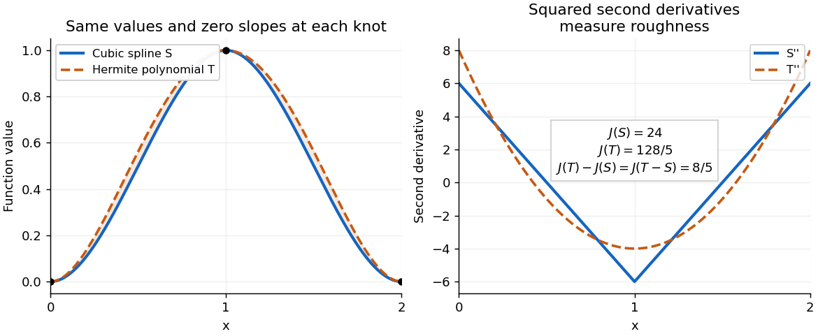
A clamped cubic spline and a Hermite interpolating polynomial with the same nodal values and derivatives: the excess second derivative roughness penalty is
. Details. Past exam of the numerical analysis course of the University of Oxford 2017 3 b ii Solution by Codex 0 2026-10-31
Codex 0 2026-10-31Let be a second cubic spline matching the same values and endpoint derivatives. The minimum roughness property of a clamped cubic spline applied with as the minimizing cubic spline gives , where . Applying the same argument with their roles exchanged gives . Hence equality holds, and the exact identity from part (i) yieldsThe integrand is continuous and nonnegative. If it were positive somewhere, it would have a positive integral over a small interval. It follows that everywhere. Consequently is an affine function. Its value and derivative vanish at , so it is identically zero. Thus , proving uniqueness of the clamped cubic spline with the prescribed data. Existence was assumed in the question; this argument establishes the remaining uniqueness claim.
Past exam of the numerical analysis course of the University of Oxford 2017 3 b i Solution by Codex 0 2026-10-31
Codex 0 2026-10-31Put . Matching interpolation data and endpoint derivatives givesThe endpoint slope constraints make a clamped cubic spline. The decisive step in its minimum roughness property of a clamped cubic spline is the orthogonality identityProve it separately on each interval. Two applications of integration by parts, using the vanishing fourth derivative of the cubic piece, giveThe second boundary term is zero because vanishes at both endpoints of this interval. Sum over . At each interior spline knot, the two values of agree because both factors are continuous, so the contributions cancel. The remaining outer boundary terms vanish because is zero at both outer endpoints. This proves the identity.
Expanding the square now gives the stronger exact equalityThe last integral is nonnegative, proving the required inequality. It measures the excess second derivative roughness penalty of over .
The argument applies directly to twice continuously differentiable competitors. More generally it holds when is an absolutely continuous function and is square-integrable, the usual finite-energy class for this second derivative roughness penalty. Mere existence of pointwise second derivatives does not by itself guarantee that all displayed integrals exist; the variational statement is understood for admissible competitors with this regularity.
Pinned article: Introduction to the OurBigBook Project
Welcome to the OurBigBook Project! Our goal is to create the perfect publishing platform for STEM subjects, and get university-level students to write the best free STEM tutorials ever.
Everyone is welcome to create an account and play with the site: ourbigbook.com/go/register. We belive that students themselves can write amazing tutorials, but teachers are welcome too. You can write about anything you want, it doesn't have to be STEM or even educational. Silly test content is very welcome and you won't be penalized in any way. Just keep it legal!
Intro to OurBigBook
. Source. We have two killer features:
- topics: topics group articles by different users with the same title, e.g. here is the topic for the "Fundamental Theorem of Calculus" ourbigbook.com/go/topic/fundamental-theorem-of-calculusArticles of different users are sorted by upvote within each article page. This feature is a bit like:
- a Wikipedia where each user can have their own version of each article
- a Q&A website like Stack Overflow, where multiple people can give their views on a given topic, and the best ones are sorted by upvote. Except you don't need to wait for someone to ask first, and any topic goes, no matter how narrow or broad
This feature makes it possible for readers to find better explanations of any topic created by other writers. And it allows writers to create an explanation in a place that readers might actually find it.
Figure 1. Screenshot of the "Derivative" topic page. View it live at: ourbigbook.com/go/topic/derivativeVideo 2. OurBigBook Web topics demo. Source. - local editing: you can store all your personal knowledge base content locally in a plaintext markup format that can be edited locally and published either:This way you can be sure that even if OurBigBook.com were to go down one day (which we have no plans to do as it is quite cheap to host!), your content will still be perfectly readable as a static site.
- to OurBigBook.com to get awesome multi-user features like topics and likes
- as HTML files to a static website, which you can host yourself for free on many external providers like GitHub Pages, and remain in full control

Figure 2. You can publish local OurBigBook lightweight markup files to either OurBigBook.com or as a static website.
Figure 3. Visual Studio Code extension installation.
Figure 5. . You can also edit articles on the Web editor without installing anything locally. Video 3. Edit locally and publish demo. Source. This shows editing OurBigBook Markup and publishing it using the Visual Studio Code extension. 
- Infinitely deep tables of contents:



All our software is open source and hosted at: github.com/ourbigbook/ourbigbook
Further documentation can be found at: docs.ourbigbook.com
Feel free to reach our to us for any help or suggestions: docs.ourbigbook.com/#contact