At $q=4$,This is an overestimate, with signed quadrature errorThe relative error is $(1/720)/(1/30)=1/24$, approximately $4.17\%$. The quartic polynomial $y^4$ lies beyond the degree of precision of a quadrature rule of Simpson's rule, so the exactness of the previous cases no longer applies.

At $q=3$,The $y$ factor is now a cubic polynomial. Simpson's rule still integrates it exactly because its degree of precision of a quadrature rule is three. Exactness of tensor-product quadrature depends on the polynomial degree in each variable, rather than their sum.

At $q=2$, the preceding tensor-product quadrature givesBoth factors of the separable integrand are quadratic polynomials, so exactness follows directly from the construction of Simpson's rule.

The orthonormal columns satisfy $\Vert a{\Vert }_2=\Vert b{\Vert }_2=1$ and $a^{T}b=0$. By part (i), $Q_{1}a=e_1$. A product of orthogonal matrices is an orthogonal matrix, since $Q_1^T{Q}_1=I$. ConsequentlyThe last expression is the first coordinate of the transformed second column. Thus the first row isThe one in the first entry uses the nonnegative retained-coordinate convention. A different consistent sign convention could give $(-1,0)$ instead; the second entry must still be zero by preservation of the inner product.

Put $C=Q_{1}A$ and write its second column as $v$. For $n\ge 3$, takewhere each angle is computed from the current second column, in the right-to-left application order. These Givens rotations eliminate its entries in rows $3,\dots ,n$ by accumulating their Euclidean norm in row two.

Each rotation acts only on rows with indices at least two. The first column of $C$ is $\Vert a{\Vert }_2{e}_1$, whose entries in all those rows are zero. Mixing two zeros leaves them zero, and row one is untouched. Thus the first column is unchanged. The resulting matrix has the formThis verifies both required properties, including the case of zero second-column tail. When $n=2$ there are no rows to eliminate: take $Q_2=I_2$, the empty product. No sign change of $v_2$ is required in that case. Each Givens row-pair update preserves previously eliminated columns, which is the central invariant of QR decomposition by Givens rotations.

Apply the product from right to left, choosing every Givens rotation from the current first column. First $J(1,2)$ replaces $(a_1,a_2)$ by $(\sqrt{a_1^2+a_2^2},0)$. Next $J(1,3)$ combines that retained entry with $a_3$ and sets the third entry to zero. Inductively, after eliminating coordinates $2,\dots ,k$, the first coordinate isand coordinates $2,\dots ,k$ are zero. Later Givens rotations involve only coordinate one and a new coordinate, so those zeros remain zero. Thereforewhere $e_1$ is the first standard basis vector. The zero vector is included by choosing the identity matrix for every zero pair. The nonnegative sign follows from the convention fixed in part (c)(ii). This is the first-column stage of QR decomposition by Givens rotations.

Let $r=\sqrt{x_i^2+x_j^2}$. If $r>0$, choose $\theta$ so thatSuch an angle exists because the two ratios have squared sum one. Then the changed coordinates areAll other coordinates satisfy $y_k=x_k$. If $r=0$, both input coordinates are zero; take $\theta =0$, giving the identity matrix on this pair. In all cases,This fixes a nonnegative retained coordinate and handles division by zero explicitly. For floating-point computation, the stable construction of a Givens rotation uses scaled Euclidean norm evaluation to avoid unnecessarily overflowing or underflowing the squares.

Choose the following consistent sign convention. The Givens rotation $J(i,j,\theta )$ equals the identity matrix except for the block on coordinates $i,j$:Thus it changes only the $i$th and $j$th coordinates of a vector. Write $c=\cos \theta$, $s=\sin \theta$. Its two-coordinate block satisfiesAll remaining coordinates are unchanged, so $J^{T}J=I_n$. Hence every such Givens rotation is an orthogonal matrix. With this convention the two-coordinate rotation matrix rotates through angle $-\theta$.

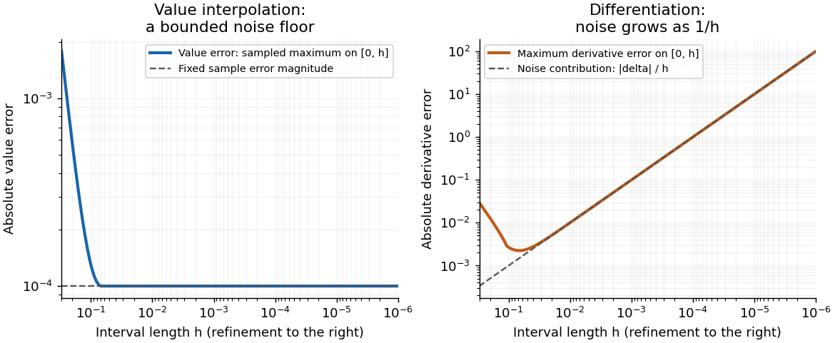
Write ${\tilde{p}}_1$ and $\tilde{q}$ for the quantities computed from the perturbed second sample. The endpoint linear interpolation and its derivative areCompare them on their interpolation interval $0\le x\le h$, with fixed $a>0$. Put $x=th$, $0\le t\le 1$. The Taylor series of the sine gives, uniformly in $t$,Here the second equality compares with $f^{\prime }(0)=a$. More generally, the exact derivative is $f^{\prime }(th)=a\cos (ath)$ andThe input perturbation itself changes the value interpolant by exactly $aϵx/h$, and changes its derivative by exactly $aϵ/h$. ThusFor fixed nonzero $ϵ$, the value approximation has a bounded noise floor: its maximum error approaches $a|ϵ|$, and at $x=h$ that error is exactly $a|ϵ|$. It does not converge uniformly to the exact values as $h\to 0$. However, it does not amplify the absolute sample perturbation on $[0,h]$. The derivative error instead grows without bound like $a|ϵ|/h$.

With exact samples, $ϵ=0$, both approximations do converge on the shrinking interval: the value error is $O(h^3)$ for this particular sine, and the derivative error is $O(h^2)$. With step-dependent noise, value convergence requires $ϵ(h)\to 0$, whereas derivative convergence requires the stronger $ϵ(h)=o(h)$, where $o$ denotes little o notation.

This is noise amplification by differentiation of a linear interpolant. Value interpolation has an absolute perturbation bound independent of $h$ on the sampled interval. Numerical differentiation has a perturbation factor $1/h$, expressing the ill-posedness of numerical differentiation from values with fixed absolute uncertainty. The amplification follows from the mathematical data map even in exact arithmetic; it is distinct from additional roundoff error in a particular implementation. For fixed $x$ outside $[0,h]$, the operation becomes extrapolation, and the value perturbation $aϵx/h$ can also diverge.

The remainder in part (b) involves an unspecified $\xi =\xi (x)$. Its existence for every $x$ does not ensure a differentiable selection. Even if such a selection existed and $f$ had an additional derivative, the product rule and chain rule would giveThe first term cannot be discarded or bounded from the given information. Neither $f^{(n+2)}$ nor ${\xi }^{\prime }$ is supplied by the original theorem.

For an explicit demonstration, interpolate the cubic polynomial $f(x)=x^3$ at zero and one. Then $p_1(x)=x$, andDifferentiating correctly givesTreating the remainder coefficient $x+1$ as a constant would omit $x(x-1)$ and give a wrong answer at every interior point. An existential intermediate point cannot be frozen when differentiating. Part (i) instead applies Rolle's theorem directly to the polynomial interpolation error.

Assume $f\in C^{n+1}[a,b]$ and reorder the interpolation nodes increasingly as $x_0<\cdots <x_n$. The polynomial interpolation error $e=f-p_n$ vanishes at all of them. Rolle's theorem suppliesThese $n$ points are distinct because their containing intervals are disjoint. Thus $q=p_n^{\prime }$ is a polynomial of polynomial degree at most $n-1$ that interpolates the function $f^{\prime }$ at the interpolation nodes ${\eta }_1,\dots ,{\eta }_n$.

Apply the polynomial interpolation error theorem to $f^{\prime }$ with these $n$ interpolation nodes. Since the $n$th derivative of $f^{\prime }$ is $f^{(n+1)}$, for every $x\in [a,b]$ there is a ${\xi }_x\in (a,b)$ withFor $x={\eta }_i$ the equality is zero on both sides; otherwise the same auxiliary-function and repeated-Rolle's theorem proof applies. This also covers $n=1$, where $q$ is a constant polynomial and the proof is the ordinary mean value theorem for $f^{\prime }$.

Writing $M={\max }_{[a,b]}|f^{(n+1)}|$ gives the genuine error boundThe first formula is sharper, but its intermediate interpolation nodes depend on $f$; the last bound eliminates those unknown locations. This is derivative interpolation error from Rolle points.

Use the nonpolynomial function $f(x)=1+\sin x$ on $[-1,1]$. Its exact integral isbecause the sine is an odd function.

For every uniform partition of an interval with $N\ge 1$ panels, the quadrature nodes satisfy $x_{N-j}=-x_j$. Their composite trapezoidal rule quadrature weights agree, so the two sampled sine values cancel. If there is a node at zero its sine value is already zero. The constant term is integrated exactly, givingThis is symmetric trapezoidal exactness for odd functions, applied after adding a constant function so that the resulting definite integral is nonzero. It is exactness for this particular integrand, rather than a claim that every nonpolynomial function is integrated exactly.

On a partition of an interval $a=x_0<x_1<\cdots <x_N=b$, apply the trapezoidal rule separately to each panel and add:For uniform spacing $h=(b-a)/N$, this composite trapezoidal rule becomesEach interior sample occurs in two panels; their half-quadrature weights combine to $h$. The endpoint quadrature weights are $h/2$.

The trapezoidal rule is exact for every affine function $f(x)=\alpha +\beta x$, equivalently every polynomial of polynomial degree at most one: the linear interpolant is the function itself. These functions have $f^{\prime \prime }=0$, so the preceding upper bound is also zero. There is no contradiction: zero error is precisely what the bound predicts.

The degree of precision of a quadrature rule is one, since the quadratic polynomial in part (i) is not integrated exactly. This does not exclude exactness for particular higher-degree or nonpolynomial functions. For example $f(x)=(x-m{)}^3$, $m=(a+b)/2$, has zero integral and opposite endpoint values, so the trapezoidal rule also gives zero. Its second derivative is generally nonzero, making the upper bound positive; an upper bound need not be attained. Signed quadrature error can cancel.

It suffices to assume $f\in C^2[a,b]$. The polynomial interpolation error for the endpoint linear interpolant gives, for every interior $x$, some ${\xi }_x\in (a,b)$ withLet $M={\max }_{[a,b]}|f^{\prime \prime }|$, which exists by continuity of the second derivative and the extreme value theorem. Since $(x-a)(b-x)\ge 0$,Integrating this pointwise inequality and using the triangle inequality for an integral yieldsThusThis derivation does not require choosing ${\xi }_x$ as a continuous function of $x$; the pointwise upper bound is sufficient.

The constant is sharp. Take the quadratic polynomial $f(x)=(x-a{)}^2$ and write $L=b-a$. Its exact integral is $L^3/3$, its trapezoidal rule value is $L^3/2$, and $\max |f^{\prime \prime }|=2$. ConsequentlyEquality holds, so no smaller universal constant than $1/12$ works under these assumptions. This is the sharp one-panel trapezoidal error bound.

With $A_0=A$, repeat the shifted QR algorithm:The QR shift ${\mu }_k$ is chosen from $A_k$, for example its bottom-right entry or an eigenvalue of a trailing two-by-two block. Explicitly using the orthogonality of $Q_k$ givesThus each update is a matrix similarity preserving eigenvalues. Accumulate $Q_0{Q}_1\cdots Q_k$ if eigenvectors or the full reduction are wanted. Once a subdiagonal entry is negligible, block deflation in the QR algorithm separates the corresponding blocks and iteration continues on the active block.

For an efficient QR algorithm, first reduce a general real matrix to upper Hessenberg matrix by orthogonal similarities. For a real symmetric matrix, use Householder tridiagonalization; the resulting symmetric tridiagonal matrix is the usual input in this setting. These structures are preserved by suitable QR algorithm implementations and greatly reduce the work per iteration.

The output is the eigenvalues, together with an orthogonal reduction when the factors are accumulated. In the symmetric case the target is a diagonal matrix, whose diagonal entries are the real eigenvalues; the accumulated orthogonal columns are eigenvectors. For a general real matrix, the target is the real form in a Schur decomposition: an upper block triangular matrix with diagonal blocks of size one or two. The two-by-two blocks represent complex conjugate eigenvalue pairs. An arbitrary unshifted iteration need not converge, so these describe the intended converged output, with appropriate shifts and block deflation in the QR algorithm.

A QR factorization of a real $n\times n$ matrix isThus $Q$ is an orthogonal matrix and $R$ is an upper triangular matrix. It exists even if $A$ is singular; requiring positive diagonal entries of $R$ is a convenient uniqueness convention for nonsingular $A$, rather than part of the general existence statement. Over the complex numbers, replace orthogonal by unitary and transpose by conjugate transpose.

Part (a), applied to any ideal class, produces an integral ideal of positive integer norm at most $c_K$, so $c_K\ge 1$. Writing $n=[K:\mathbb{Q}]$ and using $s\le n/2$ givesFor the last inequality, write $n^n/n!={\prod }_{j=1}^n(n/j)$; the first $\lfloor n/2\rfloor$ factors are at least $2$, and the remaining factors are at least $1$. Since $\lfloor n/2\rfloor \ge (n-1)/2$, squaring yieldsAs $\pi /2>1$, the assumed upper bound $D$ forcesFor $D\ge 1$, the ceiling of the right-hand side is a valid integer $M$. If $D=0$, no number field satisfies the premise, so any positive $M$ works.

For degree $3$ there are either three real embeddings or one real embedding and one complex pair. The respective Minkowski bound for ideal classes areUnder the given discriminant bound they are at most $\frac{2}{9}\sqrt{45}<2$ and $\frac{8}{9\pi }\sqrt{45}<2$. Hence every ideal class contains an integral ideal with positive integer norm strictly below $2$, so with norm $1$. The only such ideal is ${\mathcal{O}}_L$. Therefore