For the supplied hillslope values,The Froude number is below one, but it is not extremely small numerically; the much smaller products actually multiplying inertia and the depth-gradient term justify their leading neglect. Positive flow then satisfies $u=h^{2/3}$ andIn overland flow the source is net rainfall input after infiltration into soil, with evaporation or other local losses included when important. Lateral inflow can also contribute. Negative net input must be limited by water availability once the surface dries.

Manning's uniform-flow law implies the friction slope $S_f=n^2{u}^2/R^{4/3}$ for positive downstream flow. In a wide rectangular section $A\simeq wh$ and $R\simeq h$, so $\tau l/(\rho A)=g{n}^2{u}^2/h^{4/3}$.

Scale distance with $L$, depth with $h_0$, velocity with $u_0=h_0^{2/3}{S}^{1/2}/n$, and time with $L/u_0$. Divide momentum by $gS$ to obtainThe factor $ϵ$ compares depth change over $L$ with the mean bed drop $SL$, rather than with $L$ alone. Its product with $F^2$ measures inertial acceleration relative to bed-slope forcing.

Here $s$ is downstream distance, $A$ the wetted cross-sectional area, $u$ the section-averaged downstream velocity, and $M$ the lateral water input per channel length and time. Thus $A_t$ is local water storage and $(Au{)}_s$ the divergence of discharge. Their balance is mass conservation.

The momentum terms $u_t$ and $u{u}_s$ are local and advective acceleration. The bed slope $S$ gives the downstream gravitational acceleration $gS$. Bed shear stress $\tau$ acting over wetted perimeter $l$ produces resisting force per unit mass $\tau l/(\rho A)$; the hydraulic radius is $R=A/l$. Finally $-g{\overline{h}}_s$ is the hydrostatic free-surface pressure-gradient term in the chosen bed-following description. The Saint-Venant approximation depth-averages the flow, assumes a long shallow geometry and hydrostatic pressure, and closes the boundary shear through a roughness law.

For quasi-steady enzyme kinetics at low substrate saturation, the quasi-steady-state approximation is controlled here by $\epsilon =e_0/(s_0+K_m)$, rather than by $e_0/s_0$ alone. Even with $e_0\approx s_0$, taking $K_m\gg s_0$ makes $\epsilon \ll 1$ and $\sigma =s_0/K_m=O(\epsilon )$.

After the initial fast layer $T=O(\epsilon )$, the third equation givesSince $\varphi =O(\epsilon )$, the last equation gives $(e_i{)}_T=(\varphi /\epsilon )y=O(\epsilon )$. Starting from $e_i(0)=0$, this implies $e_i=O(\epsilon )$ on bounded intervals of the slow time. The quasi-steady second equation then gives $x=s+O(\epsilon )$. In the first equation,Matching to the initial substrate value $s(0)=1$ therefore yields $\boxed{s(T)\sim e^{-T/(1+\rho )}}$. The relation $x\sim s$ is an outer approximation: it does not replace the initial layer needed to reconcile $x(0)=0$ with $s(0)=1$. Likewise the smallness of accumulated inactivated enzyme has been justified for bounded slow times, not arbitrarily long times.

The conserved total is $e_0=[E](0)$ under the chosen initial conditions. Substitute $E=e_0-X-Y-E_i$ into the equations from the previous part. This closes the subsystem for $S,X,Y,E_i$; product can be recovered afterward by integrating $\dot{P}=k_{3}Y$.

Let $k_{\Sigma }=k_{-1}+k_2$ and $K_m=k_{\Sigma }/k_1$. The required nondimensionalization is completed byIndeed $X=e_0\sigma x/(1+\sigma )$ and the free-enzyme fraction is $1-\sigma x/(1+\sigma )-y-e_i$. Substitution and division by the indicated time scale giveFor example $k_2/k_{\Sigma }=1/(1+\rho )$ explains the coefficient in the third equation. The small multiplier on the intermediate-species derivatives identifies their potentially fast adjustment relative to substrate depletion.

Write concentrations as $E,S,X,Y,E_i,P$ in this calculation. The law of mass action assigns the forward bimolecular rate $k_{1}ES$ and the first-order rates $k_{-1}X,k_{2}X,k_{3}Y,k_{4}Y$. Each species gains the rates of reactions producing it and loses those consuming it:Adding the equations for all enzyme-bearing species cancels every reaction rate, so $\boxed{E+X+Y+E_i=e_0}$. This is conservation of the total enzyme-derived material, including the inactivated form. It does not assert conservation of active enzyme: mechanism-based inhibition transfers some of that conserved material irreversibly into $E_i$.

For an experiment beginning by mixing unbound enzyme with substrate, take $\boxed{[E](0)=e_0>0,[S](0)=s_0>0,[X](0)=[Y](0)=[E_i](0)=[P](0)=0}$. The enzyme-substrate complexes, inactivated enzyme and product are initially absent. Nonzero pre-existing product could be allowed without changing the dynamics here, since it has no feedback reaction in the specified scheme.

At the crossing the angular frequency is ${\omega }_c=1$, so the limiting small-amplitude period isThis is the period of the bifurcating infinitesimal oscillation. Finite-amplitude oscillations away from the threshold need not have period exactly $4\tau$.

For a purely imaginary root $\lambda =i\omega$ with $\omega >0$, separating real and imaginary parts givesThus $\omega =1$ and $\tau =\pi /2+2\pi m$, $m\ge 0$. The first crossing isFor $0<\tau <\pi /2$ there is no root with nonnegative real part. Indeed, write $\lambda =a+ib$ with $a\ge 0$. The real equation forces $\cos (b\tau )\le 0$, hence $|b|\tau \ge \pi /2$. But the imaginary equation gives $|b|\le e^{-a\tau }\le 1$, contradicting $\tau <\pi /2$.

Differentiate the characteristic equation along the root:The imaginary roots are simple because $1+i{\tau }_c\ne 0$, and they cross into the unstable half-plane as delay increases.

One can also check the nonlinear Hopf bifurcation directly. With $\theta =\omega t$ and small amplitude $a$, substituteThe constant and second harmonics at order $a^2$ give the displayed coefficients. Put $d=\mu +{\tau }_c\nu$. At order $a^3$, absence of resonant first harmonics requires $d+1/20=0$ and $\nu +3/20=0$. HenceThe nonzero coefficient verifies a branch of small periodic solutions for $\tau >{\tau }_c$, consistent with the transverse Hopf bifurcation in the delayed logistic equation. This is the delayed logistic Hopf threshold.

Put $u=1+x$. Then $\dot{x}=-x(t-\tau )-x(t)x(t-\tau )$, so the linearization is $\dot{x}=-x(t-\tau )$. A mode $e^{\lambda t}$ gives the characteristic equation of a delay differential equationFor real $\lambda \ge 0$, the left side is nonnegative and the right side negative. The two real graphs therefore never meet there, as drawn in the figure. There is no nonoscillatory exponential instability. If stability is lost, the unstable eigenvalues must be a nonreal conjugate pair, producing oscillatory growth; absence of a positive real root alone does not imply stability.

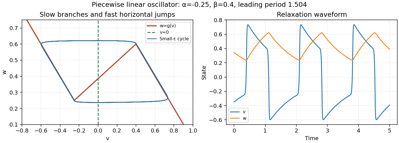
On the attracting right branch, the leading fast balance is $w=1-v$, so $\dot{w}=v=1-w$. On the left branch it is $w=-v$, so $\dot{w}=-w$. The slow travel times are thereforeBoth are positive because $w_R>w_L$. The fast jumps contribute vanishing time as $ϵ\to 0$, giving the piecewise linear relaxation-oscillator periodFor the illustrated $\alpha =-0.25$, $\beta =0.4$, the leading period is $1.5041$ in the given nondimensional time units.

The nullclines are $w=g(v)$ and $v=0$. The two outer pieces of $g$ have slope $-1$; the middle piece has positive slopeThe curve is continuous, with folds $(\alpha ,-\alpha )$ and $(\beta ,1-\beta )$. The unique equilibrium is $(0,-\alpha /(\beta -\alpha ))$. Its Jacobian matrix has trace $\mu /ϵ>0$ and determinant $1/ϵ>0$, so it is unstable. The outer branches attract the fast voltage motion.

Let $w_L=-\alpha$ and $w_R=1-\beta$. The hypothesis $\beta -\alpha <1$ gives $0<w_L<w_R<1$. The singular relaxation oscillation follows this route:

The jumps are almost horizontal in the phase plane, because $w$ changes negligibly on the fast $O(ϵ)$ time. Below $w=g(v)$, voltage increases; above it, voltage decreases; $w$ increases on the right of $v=0$ and decreases on the left. These signs provide a closed trapping region around the indicated route for sufficiently small positive $ϵ$, with the unstable equilibrium excluded, giving a periodic orbit by the planar return-map or Poincaré-Bendixson theorem argument. The continuous piecewise linear field is locally Lipschitz, so solution uniqueness is available at the corners.

The voltage nullcline is $g(v,n)=I^{\ast }$ and the recovery nullcline is $n=n_{\infty }(v)$. In the relevant region $g_n>0$, so below the voltage curve $\dot{v}>0$ and above it $\dot{v}<0$. Below the recovery curve $\dot{n}>0$, while above it $\dot{n}<0$.

For small $ϵ$, the outer voltage branches with $g_v>0$ attract fast voltage motion; the middle branch with $g_v<0$ repels it. Arrange the intersections so the equilibrium is on that middle branch, with recovery increasing along the high-voltage attracting branch and decreasing along the low-voltage attracting branch. The trajectory then drifts towards a fold, jumps rapidly to the other attracting branch at nearly constant $n$, and repeats. This is a relaxation oscillation.

The local linear stability calculation supports the construction. At an equilibrium,A sufficiently steep recovery curve gives positive determinant, while $g_v<-ϵ$ gives positive trace. Hence the equilibrium is a repeller. The bounded physical rectangle can be chosen forward invariant, and a small neighborhood of the repeller removed to give a trapping annulus. The Poincaré-Bendixson theorem then supplies a periodic orbit. These conditions can be realized because the recovery function and the applied current control the intersection and its slope; oscillation is possible, not forced for every choice.

For the illustration, ${\gamma }_K=0.1$, $H=0.8$, $v_K=0.2$, $ϵ=0.01$, $I^{\ast }=0$, $M(v)=(1+e^{-25(v-0.2)}{)}^{-1}$ and $n_{\infty }(v)=0.8/(1+e^{-20v})$. The rectangle $[-0.2,1]\times [0,0.8]$ has inward-pointing flow, and the displayed numerical trajectory realizes the folded-branch mechanism.

Write $M(v)=m^3(v)$. In the physically relevant strip $-v_K<v<1$, $0<n<H$, the zero-current nullcline satisfiesThe left side increases strictly from zero to infinity, so there is exactly one nullcline height $n=N(v)$ for each interior voltage. If $M$ is positive at the endpoints, its curve joins $(-v_K,H)$ to $(1,0)$; when low-voltage activation is idealized as exactly zero, the limiting left branch can lie on $v=-v_K$.

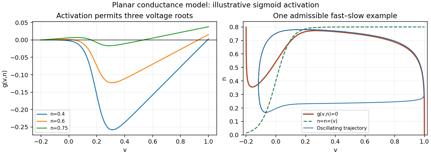
The signs of the derivatives explain its folds:At low voltage, potassium's approximately linear contribution dominates and $g_v>0$. During rapid sodium activation the last negative term can dominate, giving $g_v<0$. Once activation saturates, $M^{\prime }$ becomes small and $g_v>0$ again. This folded conductance-model nullcline has the familiar shape: the curve has descending outer branches and an ascending middle branch in the $(v,n)$ plane. Equivalently, an intermediate fixed $n$ can give three zeros of $g$ as voltage rises, with positive, negative and positive $g_v$ at those crossings.

The rapid-activation description permits this folded shape; exact fold positions depend on $M,{\gamma }_K,H,v_K$. The figure supplies an explicit admissible sigmoid example. Its right panel shows $g=0$ as well as the recovery nullcline and an oscillating trajectory.

Put $f=1-2m/r$, use proper time $s$, and denote its derivatives by dots. The timelike geodesic equations, away from the Schwarzschild coordinate singularity, arewith normalization $f{\dot{t}}^2-f^{-1}{\dot{r}}^2-r^2{\dot{\theta }}^2-r^2{\sin }^2\theta {\dot{\varphi }}^2=1$. Spherical symmetry permits an equatorial plane, $\theta =\pi /2$, and the cyclic coordinates give $\boxed{E=f\dot{t},J=r^2\dot{\varphi }}$. Normalization then gives ${\dot{r}}^2=E^2-f(1+J^2/r^2)$.

For $J\ne 0$ and $u=m/r$, $du/d\varphi =-m\dot{r}/J$. ThusAt $E=1$, $J=4m$, the right side factors as $2u(u-1/4{)}^2$. Set $q=2\sqrt{u}$, so $u=q^2/4$ and $(q^{\prime }{)}^2=(q^2-1{)}^2/8$. Integrating the regions $0<q<1$ and $q>1$ gives, up to angular shifts and time reversal,The constant $u=1/4$, or $r=4m$, is the corresponding circular timelike orbit. The hyperbolic-tangent branch lies at $r>4m$ and approaches that orbit from outside as $|\varphi |\to \infty$; the hyperbolic-cotangent branch lies at $0<r<4m$ and approaches it from inside. Near the limit $u-1/4$ decays exponentially as $e^{-|\varphi |/\sqrt{2}}$. Since $\dot{\varphi }$ tends to $J/(4m{)}^2=1/(4m)$, the limiting approach also takes infinite proper time. Neither nonconstant branch reaches and joins the circular orbit at a finite angular parameter.

Differentiating the orbit equation gives $u^{\prime \prime }=m^2/J^2-u+3u^2$. A perturbation about $u=1/4$ obeys $\delta u^{\prime \prime }=\delta u/2$, showing that the circular orbit is unstable. The two explicit curves are its separatrix branches, not ordinary small stable oscillations. For $E=1$ the energy is marginally bound, so the outer critical branch is the limiting orbit between scattering and Schwarzschild marginally bound capture from infinity. Time-reversed inner and outer branches describe the corresponding approach or departure from that unstable orbit. These are the Explicit separatrices of the marginally bound Schwarzschild orbit.

Write $f(r)=1-2m/r$ and restore $c$ for the numerical estimate. A stationary clock at radius $r$ has $d\tau =\sqrt{f(r)}dt$. Let radii $r_1$ and $r_2=r_1-h$ denote the upper and lower computers. The metric is stationary and the same two fixed spatial points exchange both signals, so each signal has the same coordinate propagation time. Therefore the interval between reception events equals the interval between emission events in coordinate time: the common delay cancels.

For upper proper running time ${\tau }_1$, the lower computer has run forIn the weak gravitational field near Earth's surface, $m=GM/c^2$ andThe lower clock runs more slowly, so its remaining work isThus about 660 micro-operations remain; the proper-time shortfall is only about $6.6\times 10^{-10}$ seconds.

Successful comparison tests the gravitational dependence of stationary proper-clock rates, specifically the radial variation of $g_{tt}$ and its weak-field gravitational redshift prediction, assuming the computers execute equally per unit proper time. It also checks that this clock effect is independent of the chosen physical clock mechanism. It does not separately verify the Schwarzschild radial metric coefficient: although light propagation uses the null metric, the identical start and finish propagation delays cancel from this particular observable. This is Gravitational redshift measured by a computation counter.

For identical fermions the full wave function is antisymmetric:In particular it vanishes when the two complete one-particle arguments coincide. Applying this to the position-only model assumes that no independent spin symmetry changes the required spatial parity.

For identical bosons the full wave function is symmetric under the particle exchange operator:In the given position-only model this is the spatial parity under the particle exchange operator. If additional spin variables are present, the symmetry applies to the complete state including them.

Under the pricing measure, the ex-dividend stock drift is $r-\delta =0.04$. ThusA direct replication holds $2e^{-\delta (T-t)}$ shares and reinvests every dividend into more shares. The share count grows at rate $\delta$, reaching two shares at expiry, with no external cash input. This payoff contains only the terminal ex-dividend stock value, unlike part (b), which also includes the separately accumulated dividends.

The diffusion associated with the displayed pricing equation is $d{\tilde{S}}_s=0.04{\tilde{S}}_{s}ds+0.2{\tilde{S}}_{s}d{W}_s$. For $Y_s=e^{-0.05s}V(s,{\tilde{S}}_s)$, Itô's formula givesThe drift vanishes by the PDE. Under the usual integrability conditions for the payoff and solution, localization and conditional expectation make $Y$ a true martingale; for polynomial-growth data the lognormal moment bounds provide the needed integrability. Applying the terminal condition yields the Feynman-Kac formulaThe printed diffusion contains an additional undefined factor $\sigma$ multiplying $0.2{\tilde{S}}_{s}d{W}_s$. If literally retained, its second-order generator coefficient would be $0.02{\sigma }^2{S}^2$, so the requested representation would correspond to that different PDE unless ${\sigma }^2=1$. The formula above uses the volatility $0.2$ specified by the stock model and by part (c).