Restrict $S$ to the vector subspace $W=\mathrm{im}T$. This restriction has kernel of a linear map $W\cap \ker S$ and image of a linear map $S(W)=\mathrm{im}(ST)$. The rank-nullity theorem on $W$ therefore givesApply the rank-nullity theorem to $T$ and $ST$ on $V$ to obtain the exact nullity of a composition identity:Since the intersection is a vector subspace of $\ker S$, its dimension is at most $n(S)$. Hence

At a locked state choose the rotating frame with ${\theta }_i^{\prime }=0$. For small phase differences, Taylor expansion gives $h({\theta }_j-{\theta }_i)-h(0)=h^{\prime }(0)({\theta }_j-{\theta }_i)+O(|{\theta }_j-{\theta }_i{|}^2)$. Let the graph Laplacian have $L_{ii}={\sum }_j{d}_{ij}$ and $L_{ij}=-d_{ij}$ for $i\ne j$. The leading locked equations areIf coupling is balanced, ${\sum }_j{d}_{ij}={\sum }_j{d}_{ji}$ for every $i$, so $1^{\mathsf{T}}L=0$. Summing over cells cancels all linear coupling terms and givesIn particular symmetric reciprocal gap-junction conductances satisfy this condition. To leading order the collective physical frequency is $1+ϵN^{-1}{\sum }_i{\xi }_i$.

The arithmetic-mean conclusion requires this extra balance assumption. The printed condition $d_{ii}=0$ alone is insufficient. For a connected directed coupling network let ${\pi }^{\mathsf{T}}L=0$, normalized by ${\pi }^{\mathsf{T}}1=1$. The valid weighted collective oscillator frequency result isFor two cells with $d_{12}=p>0$, $d_{21}=q>0$, one has $\pi =(q,p)/(p+q)$ and ${\Omega }_1=(q{\xi }_1+p{\xi }_2)/(p+q)$ at linear order. For example $p=1,q=2,{\xi }_1=0,{\xi }_2=\delta$ gives ${\Omega }_1=\delta /3$, rather than $\delta /2$, while the locked phase difference is $O(\delta )$ when $h^{\prime }(0)\ne 0$. This supplies a counterexample with arbitrarily small phase differences. It also identifies exactly why reciprocal coupling recovers the requested mean: the left null space is then spanned by the uniform vector.

Use the period-one inner product $⟨Y,V⟩={\int }_0^{1}Y(\sigma )\cdot V(\sigma )d\sigma$. Periodic integration by parts gives ${\hat{L}}^{\ast }Y=-Y^{\prime }-DF(U{)}^{\mathsf{T}}Y$. Let $Y$ span this adjoint null space and normalize ${\int }_0^{1}Y\cdot U^{\prime }d\sigma =1$. For oscillator $i$, write $s=\sigma +{\theta }_i(\tau )$. Then ${\partial }_{\tau }{u}_{i,0}={\theta }_i^{\prime }{U}^{\prime }(s)$ and ${\partial }_{\sigma }{u}_{i,0}=U^{\prime }(s)$.

The Fredholm solvability condition makes the forcing in the order-$ϵ$ equation orthogonal to $Y(s)$. Its intrinsic and frequency terms integrate to ${\xi }_i-{\Omega }_1-{\theta }_i^{\prime }$, whereVoltage-only coupling contributesThus withthe complete phase equation isPeriodicity makes these formulae independent of the absolute initial phase. The adjoint function is a phase response function; it projects a small perturbation of each state component onto its accumulated phase change. The subtraction of $h(0)$ ensures zero coupling between identical phases, as required by the original voltage differences. The source's reference to its equation (1) is read as the uncoupled cycle equation, numbered (3) on the actual page.

With $\sigma =\omega (ϵ)t$, $\tau =ϵt$, the multiscale chain rule gives $d/dt=(1+ϵ{\Omega }_1+\cdots ){\partial }_{\sigma }+ϵ{\partial }_{\tau }$. Expanding $F(u_{i,0}+ϵu_{i,1})=F(u_{i,0})+ϵDF(u_{i,0})u_{i,1}+\cdots$ gives at order oneAt order $ϵ$, moving the linearized reference dynamics to the left givesThe component sum runs over the $m$ state variables; the source uses $n$ in its first displayed sum and $m$ later. All functions for the solvability calculation are periodic in $\sigma$ with period one.

Differentiating the autonomous cycle equation $U^{\prime }=F(U)$ gives $U^{\prime \prime }=DF(U)U^{\prime }$, so $U^{\prime }$ lies in the periodic null space of $\hat{L}$. For a hyperbolic attracting limit cycle, its tangent direction has Floquet multiplier one and every transverse multiplier has modulus below one. Hence it is the only periodic direction, proving the required one-dimensional null space.

Strictly, mere nonlinear stability does not ensure this spectral assertion. In polar coordinates $\dot{r}=-(r-1{)}^3$, $\dot{\phi }=2\pi$ has an attracting unit-period cycle but neutral radial linearization at $r=1$, supplying a second periodic solution of the variational equation. Thus the intended phase reduction assumes the usual simple unit Floquet multiplier, or equivalently hyperbolic transverse attraction; this assumption is made explicit here.

The common vector field $F$ represents an identical reference cell. The small cell-specific term $ϵG_i$ represents heterogeneity of cellular properties, such as differing ion-current parameters or intrinsic oscillation rates. It is not external random noise: the displayed model is deterministic.

The Kronecker delta factors restrict coupling to the first state component, the membrane potential. Substitution gives a coupling current in the voltage equation proportional to $ϵ{\sum }_j{d}_{ij}(u_j^1-u_i^1)$, while the other state components have no direct intercellular coupling. This is the linear voltage-difference response of gap junctions. Gating and chemical variables can still change indirectly through their own coupled intracellular dynamics. The zero diagonal removes self-coupling, which would contribute zero anyway. Physical reciprocal gap-junction coupling is often symmetric, but zero diagonal alone does not impose reciprocity; that distinction matters in the final part.

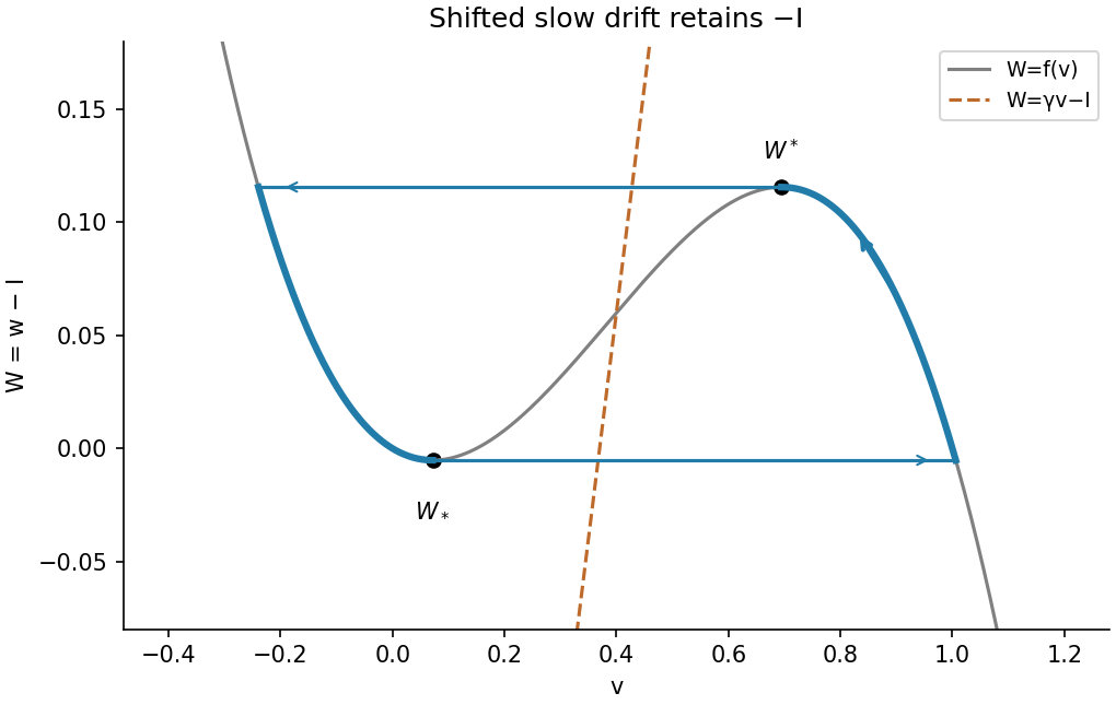
Use $W=w-I$. The nullclines become $W=f(v)$ and $W=\gamma v-I$, while the slow equation becomes $W_t=\gamma v-W-I$. The cubic has foldswith $W_{\ast }=f(v_{\ell })$ its local minimum and $W^{\ast }=f(v_r)$ its local maximum. Let $V_{-}(W)$ and $V_{+}(W)$ be the left and right attracting roots of $f(v)=W$. A line whose intersection is on the repelling middle branch permits a relaxation oscillation: upward slow travel on the right branch from $W_{\ast }$ to $W^{\ast }$, a fast jump to the left branch, downward slow travel to $W_{\ast }$, and a return jump. For sufficiently large fixed $\gamma$ this occurs for currents between the fold values $\gamma v_{\ell }-f(v_{\ell })$ and $\gamma v_r-f(v_r)$, away from the small-$ϵ$ onset layers. The straight line then crosses each outer branch beyond the relevant slow excursion, so the slow velocities have the required signs.

Neglecting the fast-jump durations, integrate $dt=dW/(\gamma V_{\pm }(W)-W-I)$ along the two slow segments. Their opposite orientations giveThe printed period omits the current shift. With the source's definition that $V_{\pm }$ solve $f(v)=w$, both denominators must retain $-I$ in the shifted coordinate. Equivalently, in the physical recovery coordinate the bounds are $I+W_{\ast },I+W^{\ast }$ and the integrand uses $\gamma V_{\pm }(w-I)-w$. The printed formula is therefore not the leading slow period for the displayed $I>0$ equations unless its notation is changed or an additional approximation justifying the omitted term is supplied.

The nullclines are the cubic $w=f(v)$ and the straight line $w=\gamma v$. At an equilibrium either $v=0$, or $\gamma =(a-v)(v-1)$. The latter quadratic has maximum $(1-a{)}^2/4$, so $\gamma >(1-a{)}^2/4$ leaves only the resting state $(0,0)$. Its Jacobian matrix isBoth eigenvalues have negative real parts; the rest state is linearly stable and asymptotically stable.

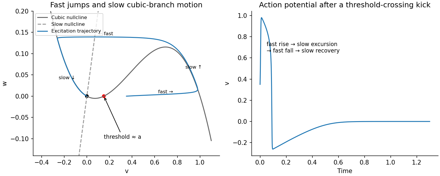
On the fast time $t/ϵ$, the recovery variable $w$ is approximately fixed. At $w\simeq 0$, the scalar fast equation has stable roots $v=0,1$ and an unstable root $v=a$. A small kick below $a$ decays towards rest; a kick above it moves rapidly towards the right attracting branch. For finite $ϵ$, the threshold is displaced from the frozen root by slow recovery, but the leading threshold mechanism is this unstable middle branch.

After the fast excitation, $w_t=\gamma v-w>0$ raises $w$ while $v$ follows the right attracting branch of the cubic. At its upper fold the branch ends and $v$ makes a fast downward jump to the left branch. Recovery then lowers $w$ slowly, with a negative undershoot in $v$, before return towards $(0,0)$. Thus the action potential time trace has rapid depolarization, a slower high-voltage excursion, rapid repolarization, and slow recovery. On the fast segments $w$ scarcely changes; on slow segments $w\simeq f(v)$ and $f^{\prime }(v)<0$. The figure shows a numerically integrated superthreshold excursion and its time trace, rather than just arrows on the nullclines.

Write $c=c_1$, $\beta =(k_{-1}+k_1^{+})/(k_1{S}_0)$ and $\kappa =k_1^{+}/(k_1{S}_0)$. Since $c_0=1-c$, the exact equations areAt the prescribed initial data $s=1,c=0$, $r_1=1$, rather than zero. The quasi-steady-state approximation would instead demand $c=s/(s+\beta )$, giving $c(0^{+})=1/(1+\beta )$. This mismatch signals an initial layer.

Set $\sigma =\tau /ϵ$ and expand $s=s_0+ϵs_1+\cdots$, $c=c_0+\cdots$. At leading order $s_0^{\prime }=0$, so $s_0=1$, while $c_0^{\prime }=1-(1+\beta )c_0$ and $c_0(0)=0$. ThusFor a more informative substrate approximation, integration of $s_1^{\prime }=-1+(1+\beta -\kappa )c_0$ with $s_1(0)=0$ givesOn the slow scale $c_{\mathrm{out}}=s_{\mathrm{out}}/(s_{\mathrm{out}}+\beta )$ and $s_{\mathrm{out},\tau }=-\kappa s_{\mathrm{out}}/(s_{\mathrm{out}}+\beta )$, with matched leading value $s_{\mathrm{out}}(0)=1$. Integrating gives $s_{\mathrm{out}}+\beta \log s_{\mathrm{out}}=1-\kappa \tau$. In the overlap $1\ll \sigma \ll 1/ϵ$, the inner complex tends to $1/(1+\beta )$ and its substrate slope matches the expansion of this outer solution. A leading composite asymptotic expansion isIt satisfies both initial values at leading order and smoothly joins the initial complex build-up to substrate depletion. The displayed $O(ϵ)$ inner substrate term records the small binding-induced initial slip if greater accuracy is wanted.

The sequential-enzyme Hill limit uses the intended distinguished limit for $n\ge 2$ holds the other rates fixed while $k_1\to 0$, $k_n\to \infty$, and $k_1{k}_n$ tends to a positive finite constant. Then for every $1\le j<n$, ${\varphi }_j={\prod }_{i=1}^j{k}_i/(k_{-i}+k_i^{+})=O(k_1)\to 0$, whereas ${\varphi }_n$ remains finite and nonzero. Hence intermediate complexes have negligible occupancy relative to the unbound and fully bound states.

In the quasi-steady-state approximation rate, all intermediate numerator and denominator terms disappear. Multiplying by $1/{\varphi }_n={\prod }_{i=1}^n{K}_i$ givesThis is the Hill equation with maximal rate $E_0{k}_n^{+}$ and effective half-saturation concentration $(\prod K_i{)}^{1/n}$. Here its power $n$ follows from the sequential binding mechanism and the suppression of intermediate states.

The phrase “$k_1{k}_n$ finite” needs this scaling interpretation for a nontrivial limiting rate. Merely bounding that product, while permitting unrelated rates to vary, does not ensure that all intermediate weights vanish relative to the terminal one. The derivation explicitly supplies the usual fixed-other-rates, positive-product assumptions. For $n=1$, the rate in the box is already the exact one-state quasi-steady-state approximation rate, without this two-endpoint limiting argument.

For an outer solution with bounded derivatives as $ϵ\to 0$, the final complex equation gives $r_n=0$. Working backwards in $0=r_i-r_{i+1}$ then gives every $r_i=0$, including $r_1$; setting only their sum to zero would not suffice. This is the quasi-steady-state approximation, valid after the initial complex-formation layer with the relevant dimensionless rate parameters held fixed.

The recurrence is $C_i=S{C}_{i-1}/K_i$, where $K_i=(k_{-i}+k_i^{+})/k_i$. Thus $C_j={\varphi }_j{S}^j{C}_0$, ${\varphi }_j={\prod }_{i=1}^j{K}_i^{-1}$. Substitution into enzyme conservation yieldsEach state $j$ produces reaction product at rate $k_j^{+}{C}_j$, soThe source's uppercase $N$ in the index range is read as the number $n$ of binding sites. This approximation preserves the total enzyme population and the different catalytic rates of the occupied states.

Besides the stated scales, set $P=S_{0}p$, $ϵ=E_0/S_0$, ${\alpha }_i=k_i/k_1$, ${\beta }_i=(k_{-i}+k_i^{+})/(k_1{S}_0)$, and ${\kappa }_i=k_i^{+}/(k_1{S}_0)$. Then $r_i={\alpha }_i{c}_{i-1}s-{\beta }_i{c}_i$, and direct substitution, remembering $d/dt=k_1{E}_{0}d/d\tau$, givesThe exact initial values are $s(0)=1$, $p(0)=0$, $c_0(0)=1$, $c_i(0)=0$ for $1\le i\le n$. The enzyme-state equations carry the small parameter because the enzyme concentration scale is small relative to the initial substrate concentration; the substrate evolves on the chosen slower depletion time scale.

Adding the ordinary differential equations for all enzyme states makes the net rates telescope:With initially unbound enzyme, this sum is $E_0$ for all time. HenceThis is enzyme conservation, not conservation of each complex individually. The reaction changes site occupancy and makes reaction product, but no event creates or destroys an enzyme molecule.

Use $S,C_i,P$ for concentrations and define net complex-formation rates $R_i=k_i{C}_{i-1}S-(k_{-i}+k_i^{+})C_i$, with $R_{n+1}=0$. The law of mass action givesEach binding event removes one free substrate molecule; each unbinding returns one; each catalytic event releases one reaction product and reduces the number of occupied sites by one. Suitable initially unbound enzyme and substrate data are $S(0)=S_0$, $P(0)=0$, $C_0(0)=E_0$, $C_i(0)=0$ for $i\ge 1$. All rates are nonnegative on the boundary of the nonnegative concentration region in the direction required to preserve it. These equations also conserve $S+P+{\sum }_{i=1}^{n}i{C}_i=S_0$, accounting for bound substrate as well as free substrate.

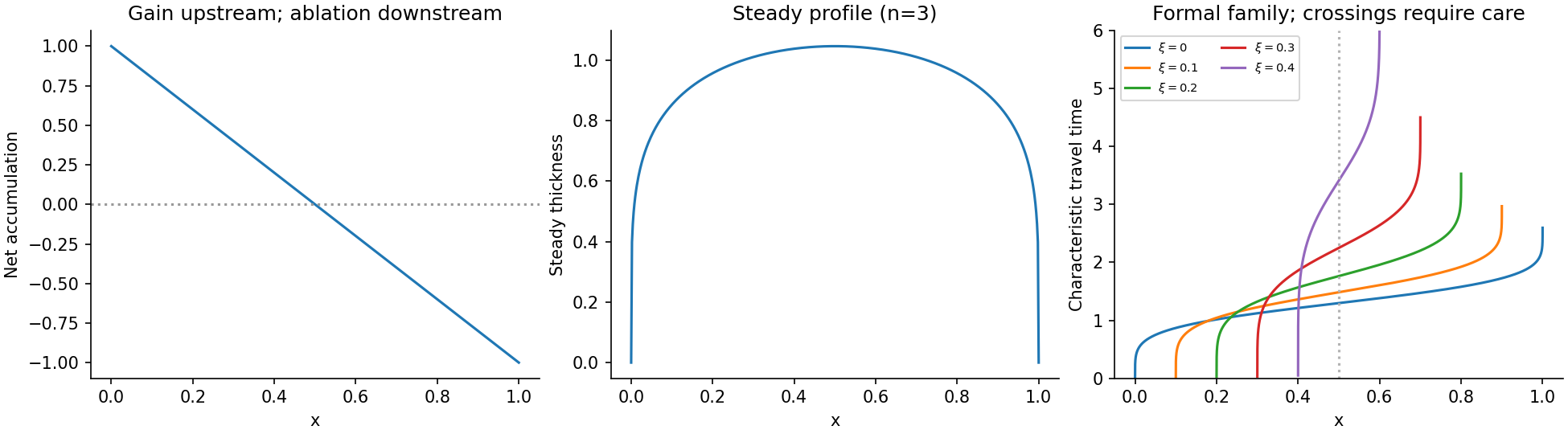
Write $A(x)=x-x^2$, $q=1/(n+2)$ and $p=(n+1)/(n+2)$. Integrating the steady mass conservation equation from the head givesFor the time-dependent first-order equation $H_t+H^{n+1}{H}_x=1-2x$, method of characteristics gives $\dot{x}=H^{n+1}$ and $\dot{H}=1-2x$. Consequently $d[H^{n+2}/(n+2)-A(x)]/dt=0$. On a characteristic starting at $(\xi ,0)$ with zero thickness,On a characteristic emitted by the boundary $x=0$, the invariant is zero and $H=H_0(x)$. The travel time of the one emitted at time zero isThe incomplete beta function is finite at both endpoints because $0<p<1$ for the physical exponents $n>0$. Before characteristic crossings, the initial-data branch and boundary-data branch have the displayed forms in the source, with the appropriate emission time $t-f(x)$ for the latter.

Glacier characteristic admissibility gives a substantive domain restriction. Factoring the invariant gives $A(x)-A(\xi )=(x-\xi )(1-x-\xi )$. A positive forward branch requiresEquivalently it is the image of this parameter domain under $(\xi ,x)\mapsto (x,t(\xi ,x))$, restricted further to regions where that map is single-valued. Characteristics cannot start with positive thickness growth at $\xi >1/2$, where the prescribed initial rate $H_t=1-2\xi$ is negative. This is why the printed piecewise expression is a formal characteristic construction, not a global nonnegative solution from a bare bed. For example for $x>1/2$, putting $L_{\xi }=1-2\xi$ givesBoth factors increase with $\xi$ there, so no positive initial-data branch exists at that $x$ for $0<t<f(x)$, contrary to a literal global reading of the first case. Compression can also make characteristics intersect; entropy solutions then require shock waves.

One can nevertheless give the exact zero-thickness endpoint locus of these formal characteristics. Let $K=f(1)=(n+2{)}^{-p}B(q,q)$. At $x=1-\xi$ the change of variable $z=\xi +(1-2\xi )y$ givesThis is the formal snout locus inferred from the given characteristic family; it retreats from $1$ towards $1/2$. It is not justified as the physical terminus of an accumulating glacier formed from zero initial ice. In particular it says nothing about a positive advancing snout at $t<K$. A physical free boundary problem must specify no ablation on a bare bed, maintain $H\ge 0$, and select an entropy solution or retain the small slope regularization. Those additional conditions are absent from the printed first-order construction. Thus a unique global physical snout trajectory cannot be claimed from that construction alone. The steady endpoint remains $x=1$. The degenerate $n=0$ limit would instead have the same endpoint time $K$ for every initial characteristic, so the inverted formula presumes $n>0$.

A typical net ice accumulation curve decreases downstream: snow gain at high elevation, zero at the equilibrium line, and negative values in the ice ablation zone. In a steady glacier with zero volume flux at its head, $Q(x)={\int }_0^{x}a(X)dX$. If its terminus also has zero volume flux, a natural glacier length $L$ is the positive root of ${\int }_0^{L}a(X)dX=0$, with the integral positive between the endpoints. Such a root requires a suitable given accumulation profile; it is not guaranteed by dimensional analysis alone.

Let $a_0$ be a representative accumulation rate and $K=A(\rho g\sin \alpha {)}^n$. ChooseUsing $x=L\hat{x}$, $H=H_{\ast }\hat{H}$, $Q=Q_{\ast }\hat{Q}$, $t=t_{\ast }\hat{t}$, $a=a_0\hat{a}$, both terms in mass conservation have scale $a_0$. The dimensionless flux isDropping hats gives the required partial differential equation. The parameter measures the surface-thickness slope correction relative to the bed slope. For the linear example $a=1-2x$, accumulation changes sign at $x=1/2$ and its integrated balance vanishes at $x=1$.

Set $G=\rho g(\sin \alpha -\cos \alpha H_x)$. For downstream shear $G\ge 0$, Glen's flow law and the no-slip boundary condition giveHere $A$ is the ice rate factor, distinct from the cross-sectional area in the river problem. Integrating this velocity profile through the thickness gives the volume flux per unit valley width:The factor $H^{n+2}$ combines the depth-dependent shear stress, integration to obtain velocity, and integration to obtain flux. If reverse shear is admitted for noninteger $n$, the signed version of Glen's flow law is $u_z=A|\tau {|}^{n-1}\tau$; the displayed unsigned power presumes the downstream regime.

Measure pressure relative to atmospheric pressure. At leading order the stress-free upper surface gives $p(H)=0$, $\tau (H)=0$. Integrating the normal balance first yieldsAt fixed $z$, $p_x=\rho g\cos \alpha H_x$. Therefore ${\tau }_z=\rho g(\cos \alpha H_x-\sin \alpha )$, independent of $z$. Integrating from $z$ to $H$ givesThis is linear in $z$, is zero at the surface, and reaches its basal value at $z=0$. In particular the surface slope modifies the shear driving; a flat upper surface relative to the horizontal eliminates it in this approximation.