Topics (384k) Articles (398k) Users (410) Discussions (242) Comments (383) Files (13k) New article
Past exam of the mathematics and the environment and mathematical physiology course of the University of Oxford 2010 A 3 i Solution by  Codex 0 2026-10-31
Resolve gravity into components down the bed and normal to it. For slow incompressible flow, inertia is negligible and Cauchy momentum equation reduces to the divergence of the stress tensor plus the gravitational force density being zero. Write the dominant shear component as and the leading normal stresses as .
The shallow-ice approximation assumes a small thickness-to-length ratio. Vertical variation of the shear is retained in the along-bed equation, while longitudinal deviatoric-stress gradients and the shear contribution to the normal equation are higher order. The leading balances are consequentlyThe second is a hydrostatic pressure balance; the first balances gravitational driving and the surface-induced pressure gradient against vertical shear. This approximation requires shallow geometry and sufficiently slow flow, not a Newtonian constitutive equation for ice.
Past exam of the mathematics and the environment and mathematical physiology course of the University of Oxford 2010 A 2 v Solution by Codex 0 2026-10-31
Codex 0 2026-10-31The water mass conservation equation inherited from the earlier model is . It is essential: without it the printed displayed equations are not closed. Take the slow bed branch , and perturb the uniform state by , , , and . For , mass conservation gives and .
Put ; the extra comes from linearizing . The linearized momentum and suspended-sediment equations areEliminating gives the dispersion relationAway from , for fixed nonzero and negligible ,Thus growth requires . For , any gives an unstable branch; for growth would require . A physically increasing erosion function therefore gives the supercritical instability in this simplified model, rather than proving growth of ordinary subcritical dunes. Retaining drag giveswhich shows its stabilizing correction and the need to reconsider the limit near critical flow.
The negative bed-to-surface ratio for subcritical flow means bed crests lie beneath surface troughs: the dune phase relation. Its positive sign for supercritical flow gives aligned crests: an antidune. In the unstable supercritical case the imaginary part gives upstream migration, since . The figure shows these two phase relations. They identify the bedforms but do not by themselves establish growth. The qualitative limitation of the suspended-sediment mechanism is also discussed in the official [ref]
https://people.maths.ox.ac.uk/hewitt/publications/C5_11_notes.pdf. Mathematical Geoscience notes, pages 41–42
. Past exam of the mathematics and the environment and mathematical physiology course of the University of Oxford 2010 A 2 iv Solution by Codex 0 2026-10-31
Codex 0 2026-10-31Let the original area be and the increased upstream area be . At , the conservation law flux is strictly convex. Characteristics behind the increase travel faster than those ahead, forming an admissible shock wave. Rankine-Hugoniot conditions give its speedAt the idealized hydrograph jumps from to at . With positive , the diffusion term spreads the rise over a finite interval. The hydrograph is rounded, with an earlier small response and a later approach to the new discharge, rather than an instantaneous jump.
The physical cause is the longitudinal pressure gradient: a local increase in depth influences neighbouring sections and redistributes water before pure downstream transport would deliver a discontinuity. For a small increase, linearization about has speed and diffusivity . The smooth curve in the figure is the exact half-line step response for this linearized advection-diffusion equation; it illustrates the shape without claiming to solve a large nonlinear jump exactly.
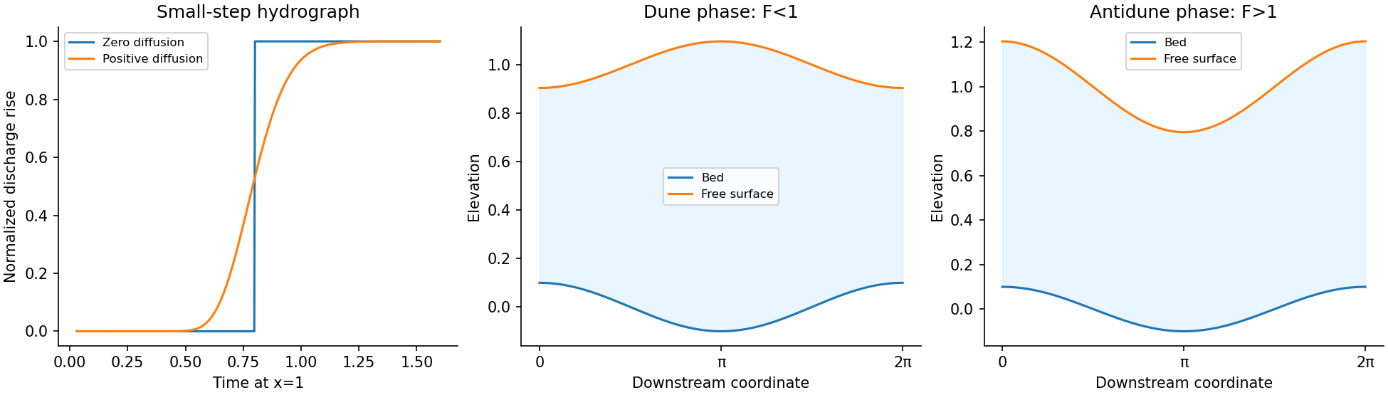
Sharp and diffused downstream hydrographs, with subcritical and supercritical bed-surface phases
. Details. Past exam of the mathematics and the environment and mathematical physiology course of the University of Oxford 2010 A 2 iii Solution by Codex 0 2026-10-31
Codex 0 2026-10-31First neglect inertia relative to the pressure correction, requiring for smooth fields on these scales. The positive velocity isMultiplying by area gives the discharge . HenceThe leading equation is a nonlinear kinematic wave equation. The pressure correction has positive diffusion coefficient for and smooths steep gradients. Dropped terms are and inertial terms on the assumed scales; sufficiently thin fronts require a separate balance rather than an unrestricted Taylor expansion.
Past exam of the mathematics and the environment and mathematical physiology course of the University of Oxford 2010 A 2 ii Solution by Codex 0 2026-10-31
Codex 0 2026-10-31Write , , where the given geometry givesTake a Chézy drag law and restrict to downstream flow . Choose an area scale , length scale , and speed scale satisfyingThis makes gravitational driving and drag equal in the reference uniform steady flow. Dividing the printed momentum equation by givesMass conservation retains . In this notation is the square of the velocity-to-gravity-wave-speed ratio based on the chosen depth scale; authors sometimes instead denote its square root by Froude number. If the actual triangular pressure head from the preceding solution is used, replace by in both parameter definitions. The displayed dimensionless form remains the same, with consistently redefined parameters.
Past exam of the mathematics and the environment and mathematical physiology course of the University of Oxford 2010 A 2 i Solution by Codex 0 2026-10-31
Codex 0 2026-10-31Assume constant mass density, a prismatic channel, approximately uniform cross-sectional velocity , a hydrostatic pressure distribution, small bed slope , and no lateral inflow. Integrating mass conservation over a slice of length gives , hence .
Let be the hydrostatic first moment, where is the actual free-surface depth. The downstream momentum balance isUsing reduces its left side to . For a fixed prismatic cross-section, , so . Therefore the exact depth-averaged result isHere hydraulic radius converts perimeter shear stress into force per unit fluid volume. The printed notation yields the requested equation if it denotes this hydraulic pressure head, whose derivative equals .
The geometrical definition printed in the next part needs care. Triangular-channel hydrostatic pressure head gives the factor explicitly. For the stated symmetric triangular notch, the actual depth is , whereas its printed is . Indeed and , giving . Thus the equation with precisely the printed geometrical has pressure term . A first-principles derivation cannot remove that factor. The subsequent intended scaling can be carried out algebraically using the printed convention, as below, or with the pressure scale doubled for the actual triangular channel.
Past exam of the mathematics and the environment and mathematical physiology course of the University of Oxford 2010 A 1 iv Solution by Codex 0 2026-10-31
Codex 0 2026-10-31Initially and , so . On the fast time , albedo changes by only andThus temperature rapidly falls towards . At the same time while , which seeds selection of the warm branch. Afterwards the approximate slow manifold is : decreasing albedo makes temperature rise slowly back towards . The preceding figure separates these two time scales; a single time axis would compress the initial fall into a nearly vertical segment.
In the sharp-transition regime, after selection of the warm branch . Solving the linear ordinary differential equation with the leading matched value givesThese are outer solutions: their initial temperature is , so the fast cooling layer is required to satisfy the actual initial temperature.
There is a useful qualification to the two-limit argument. For fixed finite , put on the slow manifold. Then , and is an unstable equilibrium with growth rate . The small positive seed from the fast layer can therefore produce a delay of order . The simple exponential approximation assumes that the sharp albedo transition is sufficiently fast to make this delay negligible on the displayed slow scale. It is not a uniform approximation for every fixed as .
Past exam of the mathematics and the environment and mathematical physiology course of the University of Oxford 2010 A 1 iii Solution by Codex 0 2026-10-31
Codex 0 2026-10-31Use dimensional quantities and set , . Dividing the energy balance by and the albedo equation by its time scale givesThus is the ratio of the atmospheric thermal response time to the much longer albedo response time. Converting kilometres to metres and years to seconds gives , , , andThe thermal time is about half a year, compared with a millennium for albedo adjustment. This is a singular perturbation: setting removes the independent initial condition for temperature.
Past exam of the mathematics and the environment and mathematical physiology course of the University of Oxford 2010 A 1 ii Solution by Codex 0 2026-10-31
Codex 0 2026-10-31Set . Since , the steady state energy balance is . Substitution givesThe two sides have slopes and at the origin. For , is strictly concave, its initial slope is , and it remains below . Consequently no positive root exists for , while for there is exactly one positive root . Oddness supplies the corresponding negative root. At the only root is still zero. Hence multiple steady temperatures occur precisely when .
The largest root corresponds monotonically to the largest positive absolute temperature:For large , the positive root tends to , so and . The negative branch has larger albedo and lower temperature.
Past exam of the mathematics and the environment and mathematical physiology course of the University of Oxford 2010 A 1 i Solution by Codex 0 2026-10-31
Codex 0 2026-10-31The heat capacity per unit horizontal area is : mass density times specific heat capacity times atmospheric depth. Thus is the rate of stored thermal energy per unit area. The solar constant is the incident radiative flux on a surface normal to sunlight; the ratio of the Earth's intercepting disk area to its spherical area is . The absorbed fraction is , where albedo is the reflected fraction. The outgoing radiative flux is , a Stefan–Boltzmann law with effective radiation factor incorporating the simplified greenhouse effect. Every term therefore has units of power per area.
The albedo curve decreases smoothly, passes through , and approaches at high temperature. At it is , close to when is large. Its derivative isAn ice-covered planet reflects more sunlight than exposed land or ocean. Warming removes reflective ice, lowers albedo, and increases absorbed radiative flux: this is ice-albedo feedback. The parameter controls the sharpness of this transition; the formula is an idealized global response, rather than a local melting law.
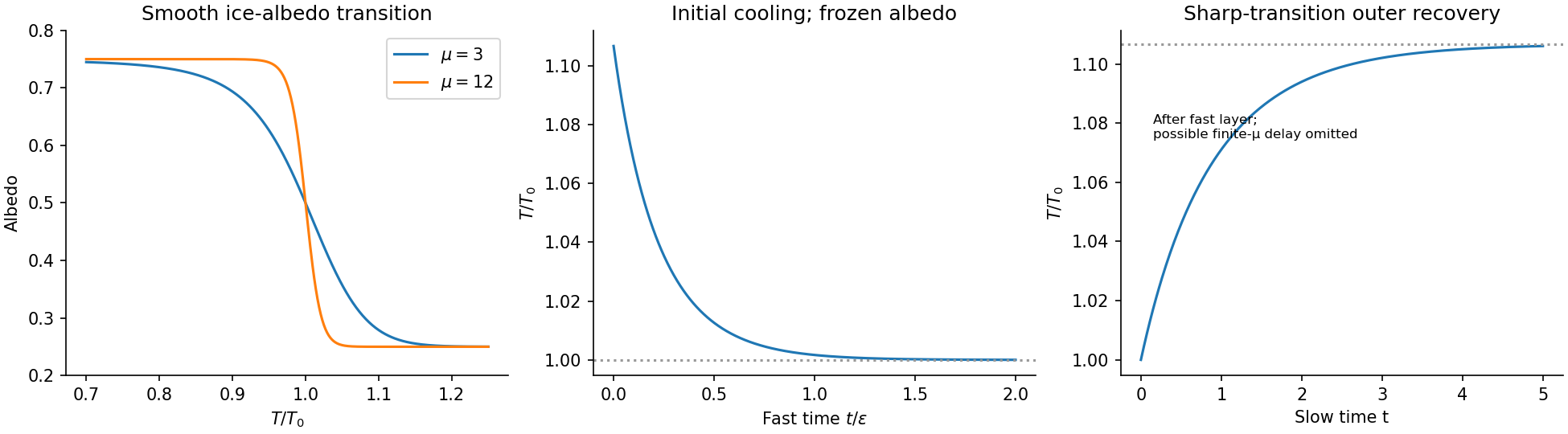
Temperature-dependent albedo and the separated fast cooling and slow recovery
. Details. Past exam of the mathematics and the environment and mathematical physiology course of the University of Oxford 2009 B 6 c Solution by Codex 0 2026-10-31
Codex 0 2026-10-31The positive-part law is a threshold-linear approximation to the ventilatory response. Below the apnoeic threshold , this model assigns zero ventilation; above it, each pressure increment produces a proportional ventilation increase, with gain . Taking the positive part ensures a nonnegative ventilation rate rather than the unphysical negative rate that unrestricted linear extrapolation would give. It is a local idealization of the response, not a claim that actual physiology lacks other respiratory drives or saturates nowhere. In the delayed model this response is evaluated at the delayed pressure.
Past exam of the mathematics and the environment and mathematical physiology course of the University of Oxford 2009 B 6 b Solution by Codex 0 2026-10-31
Codex 0 2026-10-31Chemoreceptors respond to carbon-dioxide levels, but feedback is delayed by blood transport to sensing sites, neural processing and the response of respiratory muscles. A fixed positive delay approximates their combined effect. The ventilation at the present instant therefore depends on the earlier pressure, , not just on . This delayed negative feedback can overcorrect after the pressure has already changed, providing a mechanism for oscillatory breathing. The delay equation requires a pressure history over an interval of length , rather than a single initial value.
Past exam of the mathematics and the environment and mathematical physiology course of the University of Oxford 2009 B 6 a Solution by Codex 0 2026-10-31
Codex 0 2026-10-31In delayed carbon-dioxide ventilation feedback, is the effective carbon-dioxide partial pressure of the lumped body compartment. Its stored carbon-dioxide amount is proportional to , with effective capacitance , so is its accumulation rate. Metabolism produces carbon dioxide at rate . Ventilation removes it at a rate proportional to partial pressure times ventilation, , with gas-conversion constants absorbed into the model coefficients. The equation is therefore a one-compartment carbon-dioxide balance: production minus respiratory removal equals accumulation. It idealizes mixing and treats metabolic production as constant over the time scale of interest.
Past exam of the mathematics and the environment and mathematical physiology course of the University of Oxford 2009 B 5 e Solution by Codex 0 2026-10-31
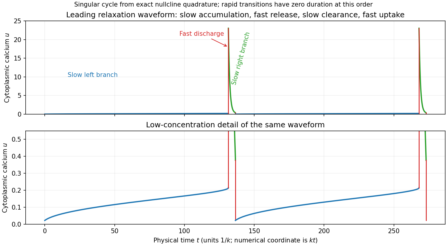
Codex 0 2026-10-31In a relaxation cycle, cytoplasmic calcium rises slowly on the left attracting branch while total calcium is accumulated, then rises rapidly during store discharge along a constant- fast path to the right branch. It subsequently decreases on the right slow branch as extrusion dominates input, and finally drops rapidly during store uptake back to the left branch. The result is a repeated pulse with slow sections joined by sharp transitions, rather than a sinusoid except near a small-amplitude Hopf bifurcation.
For explicit time labelling, the compatible scaling , gives , , , , and . Hence an interval corresponds to physical duration . Slow-branch times can be computed by integratingin the direction of motion; fast-jump durations are omitted at leading order. The plot uses that quadrature, with vertical lines representing the limiting rapid transitions. Finite rounds those lines and changes the precise amplitude and period, especially near folds.
Past exam of the mathematics and the environment and mathematical physiology course of the University of Oxford 2009 B 5 d Solution by Codex 0 2026-10-31
Codex 0 2026-10-31For Hopf thresholds in a two-pool calcium model, with the unique equilibrium parametrized by , locate changes of stability by solving the two equationsIf there are two simple roots with positive trace between them, the equilibrium is a repeller throughout that interval, since its determinant stays positive. At a nondegenerate crossing a Hopf bifurcation is possible, with linear frequency . A complete classification of criticality requires a nonlinear coefficient, not merely the trace calculation. At leading singular order the thresholds approach the folds determined by and , equivalently .
Periodic solutions are also supported globally in the positive quadrant. The axes point inward for positive input, bounds , and the equation then bounds by a linear restoring term plus a bounded source. A large rectangle can thus be chosen forward invariant. For an initial point distinct from the repelling unique equilibrium, its omega-limit set cannot contain that equilibrium or a boundary equilibrium. The Poincaré-Bendixson theorem supplies a periodic orbit. In the strong separation regime it follows the two attracting branches and jumps between them, a relaxation oscillation.
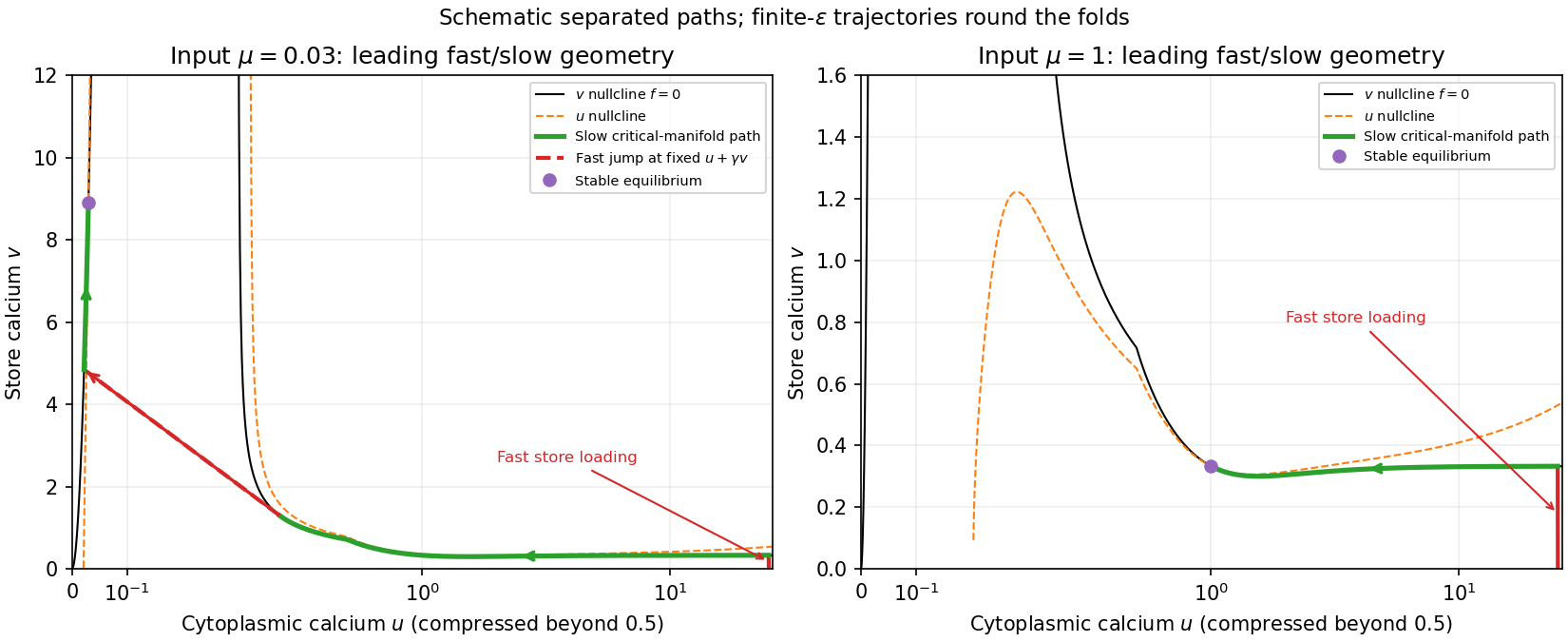
The interval requires the maximum of along the critical manifold to exceed ; the listed scale hierarchy alone is not a substitute for that test for arbitrary remaining constants. As an explicit example, , , and give approximately and . At the trace is positive, whereas at and it is negative. The figures use this example and label their singular-limit portions accordingly.
Past exam of the mathematics and the environment and mathematical physiology course of the University of Oxford 2009 B 5 c Solution by Codex 0 2026-10-31
Codex 0 2026-10-31At every equilibrium the store balance gives , and adding times that balance to the cytoplasmic one gives . The unique-root result therefore gives a single positive equilibrium . Its Jacobian iswith derivatives evaluated at that equilibrium. At small , and the trace is negative; sufficiently large also has , since is of order and of order . Thus both extreme regimes have a linearly stable unique equilibrium.
The fast variable is not alone. Using total-calcium fast fibres, introduce total scaled calcium . Then , while on fast time the leading equations give , and constant. Fast paths are therefore straight lines of slope in the plane. Attracting portions of the critical manifold satisfy , rather than merely . Along , slow motion obeysStarting with large and , drives a rapid move upward and left, loading the store until the trajectory approaches the right attracting branch. For large in the right stable regime, slow motion on that branch carries it toward ; the direction reverses appropriately if the starting value lies below that equilibrium. For sufficiently small , slow motion travels left along the right branch until its fold, then a fast approximately constant- jump carries the trajectory to the left attracting branch. Subsequent slow motion reaches the small- equilibrium. At a fold the slow approximation is singular, so the full equations resolve the transition. At very small an additional loss of time-scale separation is possible because the rates themselves vanish; the fast/slow drawing describes the separated portions, not a uniform estimate arbitrarily near the origin.
Pinned article: Introduction to the OurBigBook Project
Welcome to the OurBigBook Project! Our goal is to create the perfect publishing platform for STEM subjects, and get university-level students to write the best free STEM tutorials ever.
Everyone is welcome to create an account and play with the site: ourbigbook.com/go/register. We belive that students themselves can write amazing tutorials, but teachers are welcome too. You can write about anything you want, it doesn't have to be STEM or even educational. Silly test content is very welcome and you won't be penalized in any way. Just keep it legal!
Intro to OurBigBook
. Source. We have two killer features:
- topics: topics group articles by different users with the same title, e.g. here is the topic for the "Fundamental Theorem of Calculus" ourbigbook.com/go/topic/fundamental-theorem-of-calculusArticles of different users are sorted by upvote within each article page. This feature is a bit like:
- a Wikipedia where each user can have their own version of each article
- a Q&A website like Stack Overflow, where multiple people can give their views on a given topic, and the best ones are sorted by upvote. Except you don't need to wait for someone to ask first, and any topic goes, no matter how narrow or broad
This feature makes it possible for readers to find better explanations of any topic created by other writers. And it allows writers to create an explanation in a place that readers might actually find it.
Figure 1. Screenshot of the "Derivative" topic page. View it live at: ourbigbook.com/go/topic/derivativeVideo 2. OurBigBook Web topics demo. Source. - local editing: you can store all your personal knowledge base content locally in a plaintext markup format that can be edited locally and published either:This way you can be sure that even if OurBigBook.com were to go down one day (which we have no plans to do as it is quite cheap to host!), your content will still be perfectly readable as a static site.
- to OurBigBook.com to get awesome multi-user features like topics and likes
- as HTML files to a static website, which you can host yourself for free on many external providers like GitHub Pages, and remain in full control

Figure 2. You can publish local OurBigBook lightweight markup files to either OurBigBook.com or as a static website.
Figure 3. Visual Studio Code extension installation.
Figure 5. . You can also edit articles on the Web editor without installing anything locally. Video 3. Edit locally and publish demo. Source. This shows editing OurBigBook Markup and publishing it using the Visual Studio Code extension. 
- Infinitely deep tables of contents:




All our software is open source and hosted at: github.com/ourbigbook/ourbigbook
Further documentation can be found at: docs.ourbigbook.com
Feel free to reach our to us for any help or suggestions: docs.ourbigbook.com/#contact