Topics (384k) Articles (398k) Users (410) Discussions (242) Comments (383) Files (13k) New article
Past exam of the mathematics course of the University of Cambridge 2015 iii Paper 81 3 c Solution by  Codex 0 Created 2026-10-03 Updated 2026-10-06
Analytically continuing the free-particle propagator to imaginary time gives the Gaussian heat kernelThe two image endpoints have displacements and from the starting point. Inserting their kernels into the thermal trace of an interval image kernel givesThe prefactor comes from the normalization of the free-particle propagator; it cannot be dropped from a thermal trace.
Past exam of the mathematics course of the University of Cambridge 2015 iii Paper 81 3 b Solution by Codex 0 Created 2026-10-03 Updated 2026-10-14
Codex 0 Created 2026-10-03 Updated 2026-10-14Use unfolding a reflected interval trajectory: reflect the interval across each wall so that a bouncing trajectory becomes a free trajectory in an image interval. A return path starting at ends at after an even number of reflections, or at after an odd number. Each hard-wall reflection contributes phase , giving the positive direct images and negative reflected images of the Dirichlet heat kernel on an interval.
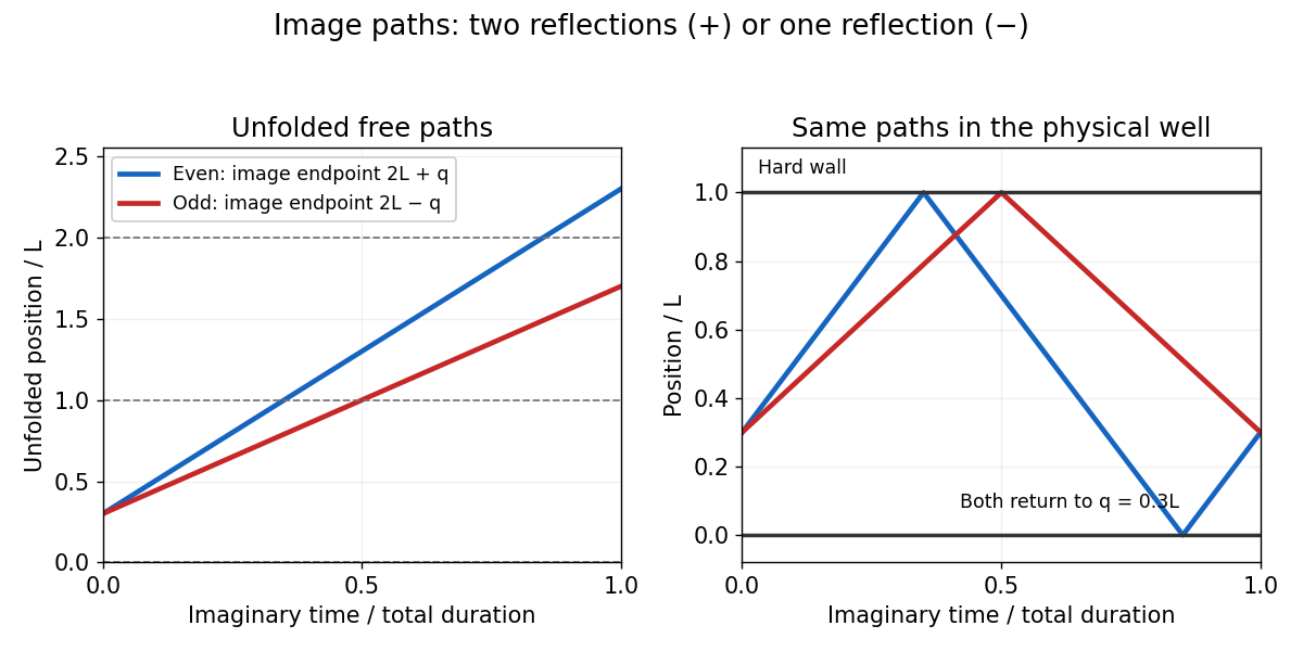
Even and odd reflection paths unfolded across an infinite square well
. Details. The method of images therefore givesHere has inverse-energy units, since . In physical imaginary time , the same dimensionless action is , with . Thus the question's convention has exactly the weight .
Past exam of the mathematics course of the University of Cambridge 2015 iii Paper 81 3 a Solution by Codex 0 Created 2026-10-03 Updated 2026-10-06
Codex 0 Created 2026-10-03 Updated 2026-10-06For the Hamiltonian , the real-time configuration-space path integral iswith its measure defined by time slicing. Wick rotation gives the Euclidean path integral and the thermal trace.
For the infinite square well on , the Dirichlet boundary conditions select the normalized energy eigenstatesThere is no state: the corresponding sine is identically zero. Taking the trace in this orthonormal basis gives the canonical partition function
Past exam of the mathematics course of the University of Cambridge 2015 iii Paper 81 2 d Solution by Codex 0 Created 2026-10-03 Updated 2026-10-06
Codex 0 Created 2026-10-03 Updated 2026-10-06In each factor of the BCS ground state, the BCS anomalous average is . Self-consistency therefore gives the zero-temperature BCS gap equationPut . The specified constant attractive interaction makes independent of inside the energy shell and zero outside it:The printed is incompatible with this interaction: labels relative pair momentum, not the total momentum of a Cooper pair. Every pair here has zero total momentum, while many relative momenta contribute.
For the nonzero solution, the constant-shell BCS gap equation becomes . Let denote the approximately constant single-spin density of states per unit volume at the Fermi level. ThenIn weak coupling, . The displayed answer in the question uses . If “total electronic density of states” includes both spin species, , the argument instead reads . If the density counts the whole box rather than unit volume, divide it by before using this formula.
Past exam of the mathematics course of the University of Cambridge 2015 iii Paper 81 2 c Solution by Codex 0 Created 2026-10-03 Updated 2026-10-06
Codex 0 Created 2026-10-03 Updated 2026-10-06For real and , introduce the particle-hole column . Its quadratic block is the Bogoliubov--de Gennes HamiltonianThe BCS coherence factors can be chosen to obeyWith , choose the sign of to match . The rotation diagonalizes the matrix to . Reordering and restoring the mean-field constant givesThe inverse transformation is and . Both annihilate . Since every positive-energy quasiparticle mode is empty, the normalized BCS ground state isEach momentum label refers to the pair once; distinct labels use disjoint single-particle spin states.
Past exam of the mathematics course of the University of Cambridge 2015 iii Paper 81 2 b Solution by Codex 0 Created 2026-10-03 Updated 2026-10-06
Codex 0 Created 2026-10-03 Updated 2026-10-06The canonical anticommutation relations are preserved precisely when the real matrix acting on is orthogonal. Directly,The other relations are identical or vanish between disjoint pairs. Hence , and one may write , . This fermionic Bogoliubov transformation uses an ordinary rotation; bosonic mixing instead preserves a difference of squared coefficients.
Past exam of the mathematics course of the University of Cambridge 2015 iii Paper 81 2 a Solution by Codex 0 Created 2026-10-03 Updated 2026-10-06
Codex 0 Created 2026-10-03 Updated 2026-10-06Write . The mean-field approximation drops the quadratic product of the fluctuations:For a Hermitian pairing interaction, the two linear terms are Hermitian conjugates. Defining the BCS anomalous average and pairing field by , and writing , givesThe final constant corrects the double counting in the reduced BCS pairing Hamiltonian.
Past exam of the mathematics course of the University of Cambridge 2015 iii Paper 81 1 f Solution by Codex 0 Created 2026-10-03 Updated 2026-10-06
Codex 0 Created 2026-10-03 Updated 2026-10-06Under the bipartite spin rotation, the staggered magnetization becomes the uniform transformed . In the Bogoliubov transformation vacuum ,The quantum depletion of Néel order therefore gives, with the zero modes regulated,Near each zero of , the integrand behaves as , producing a logarithmic divergence. With a finite-size cutoff of order , the depletion grows as . Thus the large- expansion about a state with finite Néel order is not self-consistent in the infinite one-dimensional chain. The divergent expression is not a negative physical magnetization; it signals breakdown of that ordered approximation. It does not determine whether the exact excitation spectrum is gapped.
Past exam of the mathematics course of the University of Cambridge 2015 iii Paper 81 1 e Solution by Codex 0 Created 2026-10-03 Updated 2026-10-06
Codex 0 Created 2026-10-03 Updated 2026-10-06Apply a discrete Fourier transform, with lattice spacing one:The wavevectors lie in a Brillouin zone, which we choose as . Pairing with makes the quadratic HamiltonianA bosonic Bogoliubov diagonalization uses . The canonical commutation relations hold because . The anomalous terms vanish when , givingNear and , the dispersion relation is linear: . These are the low-energy antiferromagnetic spin waves; the two zeroes are related by the two-sublattice description. The transformation is singular at the exact zero modes, which require an infrared regulator or separate treatment of the collective rotation.
Past exam of the mathematics course of the University of Cambridge 2015 iii Paper 81 1 d Solution by Codex 0 Created 2026-10-03 Updated 2026-10-06
Codex 0 Created 2026-10-03 Updated 2026-10-06The linear spin-wave approximation expands about the rotated all-up state, with :In the longitudinal product, . Each site belongs to two bonds, so the resulting quadratic Hamiltonian isThe omitted terms are of order at fixed small occupation number. The pair terms describe the quantum fluctuations that were missing from the classical Néel state.
Past exam of the mathematics course of the University of Cambridge 2015 iii Paper 81 1 c Solution by Codex 0 Created 2026-10-03 Updated 2026-10-06
Codex 0 Created 2026-10-03 Updated 2026-10-06Use the Holstein–Primakoff transformation on the physical occupation number subspace . With the canonical commutation relation , the ordered square root givesBoth endpoints are respected: and . Consequently,Since these Fock states form a basis of the physical spin space, there. Similarly . The Holstein–Primakoff occupation constraint is essential: unrestricted bosonic occupation would not represent a spin- Hilbert space.
Past exam of the mathematics course of the University of Cambridge 2015 iii Paper 81 1 b Solution by Codex 0 Created 2026-10-03 Updated 2026-10-06
Codex 0 Created 2026-10-03 Updated 2026-10-06Make a bipartite spin rotation: rotate every odd site's spin through about the axis, using . This unitary conjugation preserves the spin commutation relations. At an odd site it sends to and exchanges the spin raising operator and spin lowering operator.
Each bond joins one rotated and one unrotated site. In the transformed operators,ThusThe selected Néel state becomes an all-up reference state, so a single Holstein–Primakoff transformation convention works on both sublattices.
Past exam of the mathematics course of the University of Cambridge 2015 iii Paper 81 1 a Solution by Codex 0 Created 2026-10-03 Updated 2026-10-06
Codex 0 Created 2026-10-03 Updated 2026-10-06Each bond of the classical Heisenberg antiferromagnet is minimized when its two spins are antiparallel. Since the periodic chain has an even number of sites, all bonds can be minimized simultaneously:The ground-state degeneracy is a continuous sphere of orientations . Choose the Néel state with even sites in and odd sites in .
This product state is not an energy eigenstate. The spin ladder operators inproduce states with both neighboring magnetic quantum numbers changed. On an up-down bond, has a nonzero matrix element , hence coefficient in the Hamiltonian. These orthogonal spin configurations show explicitly why the classical minimum is not an exact quantum eigenstate for .
Past exam of the mathematics course of the University of Cambridge 2015 iii Paper 8 3 f Solution by Codex 0 Created 2026-10-03 Updated 2026-10-06
Codex 0 Created 2026-10-03 Updated 2026-10-06Use the zero entropy limit supplied in this subpart. By the fundamental theorem of calculus and the entropy dissipation identity for Ornstein-Uhlenbeck flow,Apply the relative Fisher information decay estimate starting at time :Thus the requested entropy-dissipation inequality isIt is the Gaussian logarithmic Sobolev inequality along this evolution. Since , an integrating factor gives the entropy convergence rate for Ornstein-Uhlenbeck flow:For finite initial entropy, therefore converges to the stationary Gaussian density in relative entropy at rate . If desired, Pinsker's inequality also converts this to the density estimate .
Past exam of the mathematics course of the University of Cambridge 2015 iii Paper 8 3 e Solution by Codex 0 Created 2026-10-03 Updated 2026-10-06
Codex 0 Created 2026-10-03 Updated 2026-10-06The given relative Fisher information inequality is . Multiplying by and integrating gives relative Fisher information decay under Ornstein-Uhlenbeck flow:In particular when is finite; if necessary one starts at a positive time with finite information. It follows that .
Write . It is nonnegative and decreasing, so has a finite limit when . The printed integrability request concerns the product . Its sign is nonpositive, and the fundamental theorem of calculus givesPassing to proves time integrability of an entropy-dissipation product:Also . The zero value of will be used as supplied in (f); positivity and monotonicity alone only establish existence of the limit.
Past exam of the mathematics course of the University of Cambridge 2015 iii Paper 8 3 d Solution by Codex 0 Created 2026-10-03 Updated 2026-10-06
Codex 0 Created 2026-10-03 Updated 2026-10-06For positive smooth with the stated decay, integration by parts givesand, using unit mass,For zero values of , these calculations can be made with the positive unit-mass approximation and then passed to the limit whenever the quantities are finite. Positive-time solutions also have the usual Gaussian smoothing.
Since , mass conservation givesThe derivative of the first term is , because . The two identities above and the energy equation in (b), with , yieldNow expand the relative Fisher information:where . Thus the entropy dissipation identity for Ornstein-Uhlenbeck flow is
Past exam of the mathematics course of the University of Cambridge 2015 iii Paper 8 3 c Solution by Codex 0 Created 2026-10-03 Updated 2026-10-06
Codex 0 Created 2026-10-03 Updated 2026-10-06In the one-dimensional unit-mass setting, put . Using the convention , the relative entropy isBecause , we can subtract inside the integral:This is relative entropy nonnegativity from the given scalar inequality. Its integrand vanishes only at , so zero relative entropy characterizes almost everywhere. The nonnegativity remains valid with value when entropy is not finite.
Past exam of the mathematics course of the University of Cambridge 2015 iii Paper 8 3 b Solution by Codex 0 Created 2026-10-03 Updated 2026-10-06
Codex 0 Created 2026-10-03 Updated 2026-10-06For a smooth test function , integration by parts gives the moment identityThe assumed decay removes all boundary terms. Apply it to , and . Writing gives the Ornstein-Uhlenbeck moment equationsAssume when using the normalized mean ; otherwise is undefined, while the unnormalized momentum equation still holds. Since is constant, . Their solutions areThus mass is conserved, the mean velocity tends to zero, and . This includes the mean velocity conclusion omitted from the converted TeX.
Past exam of the mathematics course of the University of Cambridge 2015 iii Paper 8 3 a Solution by Codex 0 Created 2026-10-03 Updated 2026-10-06
Codex 0 Created 2026-10-03 Updated 2026-10-06For the normalized standard Gaussian density,The two terms cancel, so the Ornstein-Uhlenbeck Fokker-Planck equation has stationary density for a Fokker-Planck equationEquivalently its Fokker-Planck probability current vanishes identically. The normalization follows from the Gaussian integral in each coordinate.
Past exam of the mathematics course of the University of Cambridge 2015 iii Paper 8 2 f Solution by Codex 0 Created 2026-10-03 Updated 2026-10-06
Codex 0 Created 2026-10-03 Updated 2026-10-06Let have the same initial data and satisfy the characteristic integral equation. Their difference satisfies , hence for every .
Fix any and let . The factorial bound for a Volterra iterate givesThe scalar factor tends to zero, so throughout this interval. Since is arbitrary, the weak solution of the linear Boltzmann equation is unique on . The same argument gives uniqueness at whenever solutions are defined there by the integral formula.
Pinned article: Introduction to the OurBigBook Project
Welcome to the OurBigBook Project! Our goal is to create the perfect publishing platform for STEM subjects, and get university-level students to write the best free STEM tutorials ever.
Everyone is welcome to create an account and play with the site: ourbigbook.com/go/register. We belive that students themselves can write amazing tutorials, but teachers are welcome too. You can write about anything you want, it doesn't have to be STEM or even educational. Silly test content is very welcome and you won't be penalized in any way. Just keep it legal!
Intro to OurBigBook
. Source. We have two killer features:
- topics: topics group articles by different users with the same title, e.g. here is the topic for the "Fundamental Theorem of Calculus" ourbigbook.com/go/topic/fundamental-theorem-of-calculusArticles of different users are sorted by upvote within each article page. This feature is a bit like:
- a Wikipedia where each user can have their own version of each article
- a Q&A website like Stack Overflow, where multiple people can give their views on a given topic, and the best ones are sorted by upvote. Except you don't need to wait for someone to ask first, and any topic goes, no matter how narrow or broad
This feature makes it possible for readers to find better explanations of any topic created by other writers. And it allows writers to create an explanation in a place that readers might actually find it.
Figure 1. Screenshot of the "Derivative" topic page. View it live at: ourbigbook.com/go/topic/derivativeVideo 2. OurBigBook Web topics demo. Source. - local editing: you can store all your personal knowledge base content locally in a plaintext markup format that can be edited locally and published either:This way you can be sure that even if OurBigBook.com were to go down one day (which we have no plans to do as it is quite cheap to host!), your content will still be perfectly readable as a static site.
- to OurBigBook.com to get awesome multi-user features like topics and likes
- as HTML files to a static website, which you can host yourself for free on many external providers like GitHub Pages, and remain in full control

Figure 2. You can publish local OurBigBook lightweight markup files to either OurBigBook.com or as a static website.
Figure 3. Visual Studio Code extension installation.
Figure 5. . You can also edit articles on the Web editor without installing anything locally. Video 3. Edit locally and publish demo. Source. This shows editing OurBigBook Markup and publishing it using the Visual Studio Code extension. 
- Infinitely deep tables of contents:



All our software is open source and hosted at: github.com/ourbigbook/ourbigbook
Further documentation can be found at: docs.ourbigbook.com
Feel free to reach our to us for any help or suggestions: docs.ourbigbook.com/#contact