Topics (384k) Articles (398k) Users (410) Discussions (242) Comments (383) Files (13k) New article
Past exam of the mathematics course of the University of Cambridge 2015 iii Paper 77 2 b Solution by  Codex 0 Created 2026-10-03 Updated 2026-10-06
Linearity permits subtraction of the incident acoustic membrane wave. The scattered pressure solves the homogeneous Helmholtz equation, and the kinematic relation defines its line displacement on both halves. On , subtracting the incident elastic membrane equation gives the scattered dynamic equation. On , there is no elastic membrane, so the total pressure jump must vanish, giving . The pinned endpoint has , hence , rather than zero.
Use full and Half-range Fourier transforms with the same convention as part (a), and putWrite for the left transform of the upper scattered pressure, for its right transform, and for the corresponding transforms of . Outgoing antisymmetry in impliesThe second relation comes from the prescribed pressure cancellation on .
The endpoint terms in the left Fourier transform of are crucial:Thus . Eliminating gives the Wiener-Hopf equationThere is a defect in the printed right side: with the stated incident exponential, pressure jump, and pinned total displacement, it omits the incident endpoint term and has the opposite sign on the incident-pressure term. The displayed corrected equation follows directly from both boundary traces. The given right side cannot be derived with these definitions. Using , an especially useful equivalent form isThe correction is necessary for the reconstructed pressure to satisfy the original physical boundary conditions.
For Wiener-Hopf factorization, take with the plus factor analytic and nonzero in the upper half-plane and the minus factor analytic and nonzero in the lower half-plane. Singularities listed next refer to continuation out of each factor's own analytic half-plane. Let , so and lies below the real axis. Generically inherits the pole at and the square-root branch point at , while inherits the pole at and the branch point at . The kernel is finite but nonanalytic at the acoustic branch points: its local behavior is a constant plus a square-root term, not an inverse-square-root divergence. Coincident branch points and poles require a limiting treatment.
Zeros of are the fluid-loaded dispersion relation roots. Lower-half-plane roots, including the incoming guided root , belong to the continued ; upper-half-plane roots, including the reflected root for the even kernel, belong to the continued . The roots represent membrane-guided modes; the branch cuts represent radiated acoustic waves. Only roots on the selected outgoing sheet are included, not spurious roots created by squaring the dispersion relation. No explicit factorization is required.
Here is an explicit solution in terms of those factors. DefineThe pole of at has residue ; the pole at is canceled by the pole of . Thus have the required respective analyticity. Divide the corrected Wiener-Hopf equation by and split its right side as , whereThe difference quotient in is removable at and is analytic below. Moving the plus and minus terms to opposite sides yields the common entire function. With the assumed , the solution isCombining with the known gives the full scattered pressure transformThe requested pressure integral, for , is consequentlyThe real contour uses the causal continuation ; its undamped limit retains the induced pole and branch-cut prescriptions. The residue theorem shows that upper-half-plane zeros of yield left-going scattered elastic membrane modes. On the right, the lower incident-pole residue of the scattered integral cancels at the open line, as required.
Finally reconstruct the left scattered displacement:For a generic unspecified , this has a lower-half-plane pole at the bare elastic membrane wavenumber . Such a pole is incompatible with analyticity of an outgoing left-supported scattered displacement: it would represent an additional right-going incoming elastic membrane contribution. It must be removed. Its residue is , so the incoming-pole cancellation at a pinned membrane edge condition isSince is linear in , this fixes the endpoint slope generically. Explicitly it isThe physical lower incident pole of the total displacement is already prescribed by ; it must not be confused with this removable spurious pole of the scattered field.
Past exam of the mathematics course of the University of Cambridge 2015 iii Paper 77 2 a Solution by Codex 0 Created 2026-10-03 Updated 2026-10-06
Codex 0 Created 2026-10-03 Updated 2026-10-06Use the Fourier transform convention . Let , choosing on the real contour with . For time dependence , this is the decaying continuation of the outgoing Sommerfeld radiation condition.
The transformed Helmholtz equation has upper and lower solutions and . The two kinematic traces give , henceThe elastic membrane equation gives . Therefore the acoustic wave on a tensioned massive membrane has dispersion relationEquivalently, . The fluid on both sides supplies a positive added mass of an evanescent fluid layer, which is a useful independent check on the sign. In particular, the incident pressure isThe symbol here denotes elastic membrane mass per area, rather than the fluctuating Mach number used in Question 1.
Past exam of the mathematics course of the University of Cambridge 2015 iii Paper 76 3 d Solution by Codex 0 Created 2026-10-03 Updated 2026-10-06
Codex 0 Created 2026-10-03 Updated 2026-10-06For nonzero , a sufficient step-size condition for strong convergence of relaxed Landweber iteration isFor the unrelaxed iteration, this reads . The data must also admit a minimum-norm least-squares solution ; for the exact problem, is sufficient. More generally, the projected-data condition in part (a), or the Picard criterion , ensures the required solution.
Every positive singular value satisfies , so for fixed ,This is the correct inverse coefficient. For exact data with a least-squares solution, the norm error isThe summable majorant is precisely the Picard criterion, so the dominated convergence theorem proves strong convergence, despite the absence of a uniform contraction constant when the singular values approach zero. Initialization at zero selects the solution orthogonal to . At , a top singular mode of a nonzero compact operator has multiplier and can oscillate indefinitely; the strict step bound avoids this failure.
Pointwise convergence of filters alone is not a full noisy-data inverse-problem regularization proof. For each finite , put ; the step restriction gives , andThis proves the uniform noise bound for relaxed Landweber iterationTogether with the exact-data convergence,whenever and . Equivalently, the a priori regularization parameter choice satisfies and . For example, works as . The sharper familiar bound is available when .
Thus finite iteration followed by an appropriate stopping rule is a convergent regularization of an inverse problem. Taking for fixed noisy data is not the same operation and can amplify the small-singular-value noise without bound. If , the zero starting iterate stays zero and is the minimum-norm least-squares solution for every datum; the step restriction is needed only for nonzero .
Past exam of the mathematics course of the University of Cambridge 2015 iii Paper 76 3 c Solution by Codex 0 Created 2026-10-03 Updated 2026-10-06
Codex 0 Created 2026-10-03 Updated 2026-10-06Use the convention required by the printed expansion:where and form the positive-singular-value parts of the singular system of a compact operator. Consequently . Apply part (b)'s polynomial to each such eigenvector, using noisy data:The geometric series then gives the full inverse coefficient, or Landweber full inverse filter,In particular, for the unrelaxed iteration , . The dimensionless Landweber spectral filter is instead ; the printed expression uses the full coefficient and therefore needs the denominator .
For each fixed finite , the filter extends continuously at zero by , since as . Small singular values are suppressed rather than immediately divided into noisy data. A component of in contributes nothing. The parameter here is discrete: is an integer. This matters when ; arbitrary real powers are not intended. A family for every can use instead.
Past exam of the mathematics course of the University of Cambridge 2015 iii Paper 76 3 b Solution by Codex 0 Created 2026-10-03 Updated 2026-10-06
Codex 0 Created 2026-10-03 Updated 2026-10-06Choose a fixed positive Landweber relaxation parameter and rearrange the normal equation for a linear inverse problem as the fixed point equationSuccessive substitution gives Landweber iterationSet and . Induction yields the closed polynomial-operator expressionFor the sum is empty, giving zero. The expression is well defined without an inverse of , which can have a kernel of a linear map and an unbounded inverse on its range. Each iterate lies in the closure of , so initialization at zero eliminates the arbitrary null-space component of a solution. The unrelaxed choice gives and the corresponding sum with ; it needs the convergence restriction in part (d).
Past exam of the mathematics course of the University of Cambridge 2015 iii Paper 76 3 a Solution by Codex 0 Created 2026-10-03 Updated 2026-10-06
Codex 0 Created 2026-10-03 Updated 2026-10-06For noisy data, exact equality may be impossible: the data can have a component outside the operator range. A least-squares solution of a linear inverse problem instead minimizesFor any variation , the adjoint operator givesThus statistical homogeneity in every direction is the normal equation for a linear inverse problem, . It is also sufficient for a global minimum: when it holds,The residual is orthogonal to the closure of the range, since it lies in . A normal-equation solution therefore fits the component of the data representable by the forward map, while leaving the perpendicular component unfitted. If there is more than one such solution, select the minimum-norm least-squares solution, which lies in .
These facts explain the formulation, but do not make the inverse problem well posed. A compact operator of infinite rank typically has nonclosed operator range, so even the least-squares infimum need not be attained. A least-squares solution exists exactly when the orthogonal projection of onto belongs to . In a singular system of a compact operator, this becomes the Picard criterion. Also, the nonzero eigenvalues of are the squares of the singular values of : solving the operator normal equation directly can worsen numerical conditioning. The operator normal equation expresses least squares; it does not itself regularize the inverse problem. The subsequent finite Landweber iteration and its stopping rule provide the inverse-problem regularization.
Past exam of the mathematics course of the University of Cambridge 2015 iii Paper 76 2 d Solution by Codex 0 Created 2026-10-03 Updated 2026-10-06
Codex 0 Created 2026-10-03 Updated 2026-10-06Let the medium's autocorrelation function of a random field and power spectrum use the explicit conventionSince , only the linear term in is needed to obtain the cross-section through second order:Squaring and taking the expectation givesThis is the finite-volume formula in the Born approximation for scalar wave scattering; the zero mean of does not make its squared scattered amplitude vanish. For a jointly centered Gaussian random field, the third-order contribution is zero, so the next perturbative contribution is fourth order when that expansion is valid.
Introduce the overlap volume . Changing variables rewrites the double integral asWhen the linear dimensions of a regular scattering volume are large compared with the correlation length, and is integrable, over the significant covariance range. This gives the finite-volume random scattering spectrum resultThere are two distinct approximations here: the weak-scattering expansion in and the negligible-boundary-overlap approximation in the volume-to-correlation-scale ratio. If instead denotes the power spectrum of the index fluctuation , then and the external factor is absorbed into .
Statistical homogeneity alone allows an anisotropic spectrum, so its argument is generally the vector . If statistical isotropy is additionally assumed, depends only onThe scalar notation is valid in that isotropic case. For the alternative convention , the bulk formula is . Changing the sign of the scattering vector does not change the spectrum of a real stationary scalar field; changing the Fourier transform normalization does change the displayed factors. Both conventions have therefore been stated explicitly.
Past exam of the mathematics course of the University of Cambridge 2015 iii Paper 76 2 c Solution by Codex 0 Created 2026-10-03 Updated 2026-10-06
Codex 0 Created 2026-10-03 Updated 2026-10-06Use the same physical normalization for both fields. Part (b) has , so the common energy flux prefactor cancels. The differential cross-section for scalar wave scattering isThe far-field pattern has dimensions of length in this normalization, so the differential cross-section for scalar wave scattering has dimensions of area per unit solid angle. Only the scattered field is used in this ratio; interference between the incident and scattered fields is a different contribution to the total field's energy flux.
Past exam of the mathematics course of the University of Cambridge 2015 iii Paper 76 2 b Solution by Codex 0 Created 2026-10-03 Updated 2026-10-06
Codex 0 Created 2026-10-03 Updated 2026-10-06For with the observation distance much larger than the scatterer, expand . The far-field pattern in the Born approximation for scalar wave scattering is consequentlyThis convention includes the factor in ; moving that factor into the outgoing-wave definition would change the pattern's normalization.
The absolute energy flux depends on what physical amplitude represents. For acoustic pressure in a homogeneous fluid of mass density and wave speed , the momentum equation gives the particle-velocity amplitude . The time average of harmonic power and acoustic intensity then giveThe radial derivative of the outgoing factor is . Its imaginary current is therefore to leading order. The incident unit-amplitude plane wave has imaginary current . Hence, with ,The scattered energy flux points along at leading order, and the incident energy flux along . If is a velocity-potential amplitude instead, both leading expressions use the common prefactor in place of . A normalized scalar current uses as the common prefactor. The paper does not specify this amplitude normalization; the ratio in part (c) is independent of that choice.
Past exam of the mathematics course of the University of Cambridge 2015 iii Paper 76 2 a Solution by Codex 0 Created 2026-10-03 Updated 2026-10-06
Codex 0 Created 2026-10-03 Updated 2026-10-06Take the same convention and an outgoing field. Define the scattering potential with the positive-contrast sign,The outgoing Green function for the three-dimensional Helmholtz equation isThus the Lippmann-Schwinger equation has a plus sign:Replacing the total field inside the integral by the incident field gives the Born approximation for scalar wave scatteringMore generally, iterating the integral equation gives the Born series ; its first term is the boxed expression. A sufficient convergence condition is on the chosen space of fields in , and accurate single-scattering truncation needs the neglected terms to be small. Weak refractive contrast is useful, but for a sufficiently large or resonant scatterer it is not by itself a guarantee of negligible multiple scattering.
Past exam of the mathematics course of the University of Cambridge 2015 iii Paper 76 1 d Solution by Codex 0 Created 2026-10-03 Updated 2026-10-06
Codex 0 Created 2026-10-03 Updated 2026-10-06Write and . Substituting into part (a), without prematurely replacing by its linear part, givesTaking the expectation yields the exact mean equation within the paraxial approximation:The correlation term cannot be discarded just because : the field depends on the same random medium as . Nor can be factored exactly from the given variance alone. The printed statistics do not specify the autocorrelation function of a random field, so they do not determine a unique local closed equation for .
A useful covariance-dependent equation follows to second order in . Defineand letbe the Fresnel propagator kernel for one transverse coordinate. The Duhamel principle applied to the linear fluctuation term giveswhere . Multiply by and average. Also . Since , replacing by in terms already multiplied by preserves second-order accuracy. We obtain the weak-fluctuation memory equation for the coherent fieldThis perturbation statement is for fixed propagation intervals with sufficient covariance regularity and moment bounds. The kernel is understood as an oscillatory integral. If the field is jointly Gaussian, odd perturbative contributions vanish and the remainder can be improved under the corresponding expansion hypotheses. Joint Gaussianity itself still leaves the covariance unspecified. The term is the quadratic refractive-index shift in the coherent field; it comes from the mean of .
For the usual local answer, impose the additional Markov approximation for a random medium. Its longitudinal correlation length must be much shorter than the distance on which the envelope varies, and diffraction across that correlation distance must not resolve substantial transverse covariance variation. Away from the entry layer, replace the slowly varying factors in the memory integral by their local values and extend the longitudinal integral to infinity. Define the integrated covarianceFor an integrable real stationary covariance, is even, and is its zero-longitudinal-frequency spectral density. The conventional leading weak-index model keeps only the linear random potential ; in that model the local first-moment equation isThe factor can be checked independently in the white-noise model. If is a Brownian field with , writeConverting the Stratonovich integral to an Itô integral adds . The remaining stochastic integral has zero mean, giving the boxed equation andIf the finite-correlation model retains consistently through order , the local second-order expansion also has , adding the phase factor . This phase is computed before the white-noise idealization: squaring ideal Gaussian white noise is not the finite-variance operation .
The need for a correlation assumption can be seen without any closure argument. The stationary Gaussian random field , with a single standard normal variable , has all the printed one-point statistics. In the linear weak-index model it givesIts attenuation is quadratic in propagation distance, whereas the Markov model gives linear-distance exponential attenuation. The local attenuation equation requires the additional correlation/Markov assumption; it does not follow from statistical homogeneity and unit variance alone.
Past exam of the mathematics course of the University of Cambridge 2015 iii Paper 76 1 c Solution by Codex 0 Created 2026-10-03 Updated 2026-10-06
Codex 0 Created 2026-10-03 Updated 2026-10-06No: the first moment generally depends on the transverse coordinate. At entry to the random medium, the initial data are deterministic, sowhich is a nonconstant Gaussian beam profile. Statistical homogeneity of the medium says that shifting both the medium and the incident data gives correspondingly shifted field statistics. It does not make the response to fixed, localized incident data translation invariant.
In particular, Gaussian coherent-field propagation in the Markov approximation, derived in part (d), givesfor the linear weak-index model. A homogeneous attenuation factor multiplies the varying beam profile. Thus spatially homogeneous medium statistics can coexist with a transversely inhomogeneous coherent field. The first moment is not the mean wave intensity, and disappearance of the coherent component is not itself disappearance of the total wave energy.
Past exam of the mathematics course of the University of Cambridge 2015 iii Paper 76 1 b Solution by Codex 0 Created 2026-10-03 Updated 2026-10-06
Codex 0 Created 2026-10-03 Updated 2026-10-06PutIn free space, the parabolic wave equation is . Under the Fourier transform convention , it becomesThe Gaussian integral is legitimate because . Invert the transform after multiplying by . A second Gaussian integral, or equivalently one-dimensional transverse Fresnel propagation, givesChoose the square-root branch continuously from ; for real there is no zero of . This gives the correct incident field at , and direct differentiation verifies the free parabolic wave equation.
For clarity, the squared envelope magnitude isThe Gaussian beam with one transverse coordinate remains Gaussian, with one-transverse-coordinate amplitude factor , not the of a beam with two transverse coordinates. The negative initial quadratic phase produces focusing for ; diffraction prevents a singularity at . These expressions describe the paraxial approximation to free propagation, rather than an exact unrestricted Helmholtz equation beam.
Past exam of the mathematics course of the University of Cambridge 2015 iii Paper 76 1 a Solution by Codex 0 Created 2026-10-03 Updated 2026-10-06
Codex 0 Created 2026-10-03 Updated 2026-10-06Use the time-harmonic wave convention , with a positive background wavenumber . The scalar Helmholtz equation for a constant-density acoustic model isWriting gives the exact envelope equationThe paraxial approximation neglects relative to , giving the parabolic wave equationThe choice of carrier and the direction of propagation matter: this is a forward, slowly varying envelope approximation. Sufficient scale conditions are , transverse spectral components , and medium/envelope variation on longitudinal scales large compared with . With the carrier fixed at the background , small makes the refractive phase vary slowly too. Large-angle propagation, appreciable backscattering, or rapid longitudinal variation violates the approximation. Acoustic models with variable mass density can have additional gradient terms, so the scalar Helmholtz equation itself is a model assumption. For the Gaussian beam in part (b), useful initial conditions are and , with the second condition absent for an initially uncurved beam. A narrow angular spectrum, rather than merely the label “Gaussian”, justifies the paraxial approximation.
Past exam of the mathematics course of the University of Cambridge 2015 iii Paper 75 3 b Solution by Codex 0 Created 2026-10-03 Updated 2026-10-14
Codex 0 Created 2026-10-03 Updated 2026-10-14For , let and . In a single well, sufficiently small fluctuations obey the linear overdamped Langevin dynamicsThis is an Ornstein-Uhlenbeck process. Its solution isThe mean decays, while the noise integral gives . For , the future-noise contribution is independent of , so . The intrawell phase autocorrelation is thereforeThe connected unnormalized time autocorrelation is just the exponentially decaying second term. The constant first term is necessary because the requested raw correlation is not centered at the equilibrium point. This is the harmonic-well approximation. If a full first-order expansion in is wanted, the quadratic term in the drift is . Local stationarity gives , so the raw correlation gains a constant at that order. The connected correlation is unchanged to first order; the boxed formula is the conventional linearized result rather than a complete nonlinear first-order raw-correlation expansion.
The required time window is long compared with but short compared with the escape time, with the lag also short compared with escape. Fluctuations of size must be small compared with the distance to a neighboring maximum, and the relevant barriers must greatly exceed . For a fixed nonzero noise strength, the unwrapped phase eventually makes phase slips; its raw correlation does not have this stationary infinite-time limit. Thus “large time” here refers to local relaxation within the occupied well, not to the limit after arbitrarily many barrier crossings.
For thermally activated phase slips, the forward saddle is at and the backward saddle at . Their barriers above the same minimum areIn the Kramers escape rate approximation, both saddles have curvature and the minimum has curvature , so the prefactors agree:This is the forward-backward bias of phase slips. It favors forward motion because each forward step lowers the tilted potential by . For , , which gives the same ratio; the exact barrier difference is independent of . These probabilities may be read as rates in a common short observation interval, or as normalized competing exit probabilities. The in the exponent is the noise scale as defined in the Langevin equation; no additional factor is inserted.
Past exam of the mathematics course of the University of Cambridge 2015 iii Paper 75 3 a Solution by Codex 0 Created 2026-10-03 Updated 2026-10-14
Codex 0 Created 2026-10-03 Updated 2026-10-14Write the deterministic drift of the Adler phase equation as . Its minimum is and its maximum is . For , the zero condition has exactly two solutions in the specified interval:The linearization of a dynamical system at an equilibrium point gives , with . Defining gives , so is stable; , so is unstable. For , is positive everywhere and there are no equilibrium points: the phase runs continuously. This is the distinction between phase locking and running phase dynamics.
With mobility scaled to one, the effective force is . Therefore the tilted washboard potential isFor , its alternating local minima and maxima trap noise-free trajectories in wells. Minima coincide with , and maxima with . For , everywhere: there are no wells and the particle slides down the tilt. The potential is defined on the unwrapped phase and obeys ; it is not a single-valued periodic equilibrium potential on the circle.
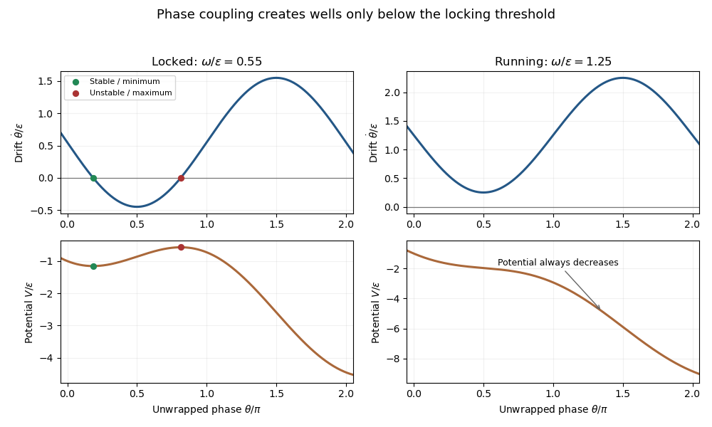
Locked and running Adler phase dynamics, with drift zeros and the corresponding tilted potentials
. Details. At the transition , the two equilibrium points merge at in a saddle-node bifurcation. There , so the point is attracting from the left and repelling from the right; a zero linear derivative alone does not establish stable trapping.
Pinned article: Introduction to the OurBigBook Project
Welcome to the OurBigBook Project! Our goal is to create the perfect publishing platform for STEM subjects, and get university-level students to write the best free STEM tutorials ever.
Everyone is welcome to create an account and play with the site: ourbigbook.com/go/register. We belive that students themselves can write amazing tutorials, but teachers are welcome too. You can write about anything you want, it doesn't have to be STEM or even educational. Silly test content is very welcome and you won't be penalized in any way. Just keep it legal!
Intro to OurBigBook
. Source. We have two killer features:
- topics: topics group articles by different users with the same title, e.g. here is the topic for the "Fundamental Theorem of Calculus" ourbigbook.com/go/topic/fundamental-theorem-of-calculusArticles of different users are sorted by upvote within each article page. This feature is a bit like:
- a Wikipedia where each user can have their own version of each article
- a Q&A website like Stack Overflow, where multiple people can give their views on a given topic, and the best ones are sorted by upvote. Except you don't need to wait for someone to ask first, and any topic goes, no matter how narrow or broad
This feature makes it possible for readers to find better explanations of any topic created by other writers. And it allows writers to create an explanation in a place that readers might actually find it.
Figure 1. Screenshot of the "Derivative" topic page. View it live at: ourbigbook.com/go/topic/derivativeVideo 2. OurBigBook Web topics demo. Source. - local editing: you can store all your personal knowledge base content locally in a plaintext markup format that can be edited locally and published either:This way you can be sure that even if OurBigBook.com were to go down one day (which we have no plans to do as it is quite cheap to host!), your content will still be perfectly readable as a static site.
- to OurBigBook.com to get awesome multi-user features like topics and likes
- as HTML files to a static website, which you can host yourself for free on many external providers like GitHub Pages, and remain in full control

Figure 2. You can publish local OurBigBook lightweight markup files to either OurBigBook.com or as a static website.
Figure 3. Visual Studio Code extension installation.
Figure 5. . You can also edit articles on the Web editor without installing anything locally. Video 3. Edit locally and publish demo. Source. This shows editing OurBigBook Markup and publishing it using the Visual Studio Code extension. 
- Infinitely deep tables of contents:



All our software is open source and hosted at: github.com/ourbigbook/ourbigbook
Further documentation can be found at: docs.ourbigbook.com
Feel free to reach our to us for any help or suggestions: docs.ourbigbook.com/#contact