Topics (384k) Articles (398k) Users (410) Discussions (242) Comments (383) Files (13k) New article
Past exam of the mathematics course of the University of Cambridge 2015 iii Paper 74 4 d Solution by  Codex 0 Created 2026-10-03 Updated 2026-10-06
Seek a nonzero-buoyancy, separable similarity solution of the unsteady Boussinesq triangular-profile line-plume balances, using powers of distance and time. Let , allowing a time origin, and initially take distance from the virtual origin. Balancing the powers in the momentum and buoyancy equations and the entrainment balance gives the formOne way to recover the exponents is to let and . Matching the spatial powers in , and gives ; matching the time powers gives . The momentum equation then gives the powers of . In the resulting solution, is time-independent, so the storage term in the first equation vanishes exactly.
Direct substitution yields the coefficient equationsFor a rising buoyant solution , the last equation gives . The first then gives , and the second gives . The separable decaying line-plume similarity is thereforeReconstructing the physical fields confirmsFor example, and cancel; the momentum balance similarly gives .
The unshifted form uses and is defined for , with a singular zero-time limit. To give a finite solution for all , choose . The equations also permit replacing by , a plume virtual origin; at a finite physical source distance this family has flux histories proportional to . The Boussinesq approximation requires in the region modelled. This is a decaying similarity family; its time and virtual origins require source or initial data. The PDF supplies neither, so a unique forced-startup history cannot be selected from it. In particular, the singular unshifted field should not be presented as a regular solution at .
Past exam of the mathematics course of the University of Cambridge 2015 iii Paper 74 4 c Solution by Codex 0 Created 2026-10-03 Updated 2026-10-06
Codex 0 Created 2026-10-03 Updated 2026-10-06Apply volume conservation, mass conservation and vertical momentum flux balance to a slice of the triangular-profile line plume. Ambient ingestion contributes of volume and of mass per unit height and source length. The ambient is quiescent, so it supplies no leading vertical momentum. The integrated driving force is the stored buoyancy . Using the quantities from part (a), the non-Boussinesq triangular-profile line-plume balances areTogether with Batchelor entrainment, these are three equations for . They neglect viscous boundary stresses and streamwise pressure-force corrections within the integral-plume approximation.
Multiplying volume conservation by and subtracting times mass conservation cancels the ambient sources exactly, givingThis is buoyancy conservation in the homogeneous ambient; it is a consequence of the first two balances, not an additional independent equation.
Now take the Boussinesq approximation in inertia and entrainment, retaining the small density deficit in buoyancy. Then , and . ConsequentlyThe mass source is . Substitution into the mass conservation, momentum and buoyancy balances gives the unsteady Boussinesq triangular-profile line-plume balancesThese use density-weighted mass and momentum fluxes. Removing from some flux definitions while retaining it in the source would mix incompatible conventions.
Past exam of the mathematics course of the University of Cambridge 2015 iii Paper 74 4 b Solution by Codex 0 Created 2026-10-03 Updated 2026-10-06
Codex 0 Created 2026-10-03 Updated 2026-10-06The Batchelor entrainment hypothesis models turbulent ingestion of ambient fluid through the plume edges. A self-similar turbulent plume has a spreading rate proportional to its axial velocity scale; the hypothesis represents the unresolved mixing by an inward edge speed proportional to that scale. For the prescribed centreline velocity, the Boussinesq approximation givesThe entrainment coefficient is dimensionless and depends on the chosen velocity/profile convention and mixing regime. Here is the inward entrainment speed relative to the moving plume boundary, and the factor two counts its two sides.
A suitable density-corrected extension is , representing the reduction in ambient ingestion for a much lighter non-Boussinesq plume. It reduces to the boxed closure when . This is a phenomenological model, not an exact identity for arbitrary turbulent flow. Woods's non-Boussinesq plume model uses this density correction. The balances in part (c) can be written with either closure before taking their common Boussinesq limit.
Past exam of the mathematics course of the University of Cambridge 2015 iii Paper 74 4 a Solution by Codex 0 Created 2026-10-03 Updated 2026-10-06
Codex 0 Created 2026-10-03 Updated 2026-10-06At a fixed height, first determine the stored quantities per unit vertical height and per unit length along the line source. With , the triangular-profile line plume has the useful profile integralThe geometric volume is ; the mass is . The upward momentum is , while the buoyancy force is . ThusHere positive buoyancy corresponds to a rising light plume. If instead buoyancy is defined kinematically, divide by ; the density-weighted convention here is the one matching the printed equations.
Multiply each local density by the vertical velocity to obtain the fluxes through a horizontal section, still per unit source length:In particular, the stored momentum equals the mass flux , and the buoyancy flux is . The different triangular-profile factors in storage and flux must not be replaced by top-hat coefficients.
Past exam of the mathematics course of the University of Cambridge 2015 iii Paper 74 3 d Solution by Codex 0 Created 2026-10-03 Updated 2026-10-14
Codex 0 Created 2026-10-03 Updated 2026-10-14Continue with downward coordinate and . By Stokes drag law, the small-particle isolated settling velocity is . Normalize concentrations by : write . In suspension the specified independent hindered settling laws give fluxes and . The initial state is .
Two upper sedimentation shocks clear the species separately. The faster front removes large particles, leaving behind it; the small concentration is unchanged across this front because the species fluxes are independent. The slower front separates that small-only suspension from clear fluid. Their downward velocities areThere is also a growing mixed deposit at the bottom. Let its normalized solid concentrations be , with , and let its upward speed magnitude be . Applying the Rankine-Hugoniot condition to each species givesAdding these relations provesThe deposited flux is zero even though each species occupies only part of the packing: the settling law applies to the suspension, while the deposit is a separate stationary state. These jump relations determine the deposit composition from sedimentation jump conditions.
The large-particle clearing front has height and meets the mixed-deposit front at height . ThusAt this merger all large particles have entered the deposit. Only the small particles remain suspended, at normalized concentration . The new material deposited above the mixed layer is pure small-particle solid, at total concentration . Its sedimentation shock therefore has downward speedFor , the deposit top and the remaining clearing front have heightsTheir meeting, or the total solid-volume balance, givesThis is two-stage bidisperse batch sedimentation: the fast species finishes first, followed by deposition of the remaining slow species.
The final solid composition by volume, and also by mass because the particle densities are identical, isThe upper pure-small layer has thickness . As checks, accounts for all large-particle solid volume, and accounts for all small-particle solid volume, in units of . If “percentage of particles” means number rather than volume, a large sphere occupies eight times the volume of a small sphere: the mixed bottom layer contains large particles by number and small. The upper layer remains entirely small under either convention.
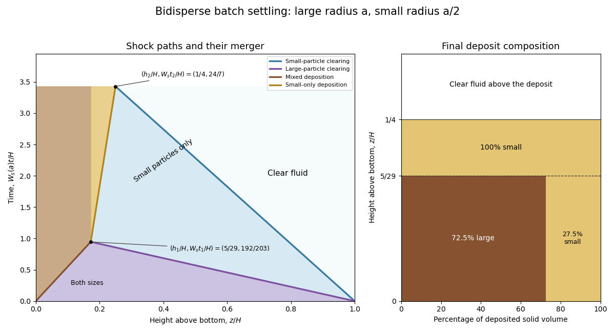
Bidisperse sedimentation: three initial shocks, merger at t1 and h1, final settling at t2 and h2, and solid-volume composition of the deposit
. Details. Past exam of the mathematics course of the University of Cambridge 2015 iii Paper 74 3 c Solution by Codex 0 Created 2026-10-03 Updated 2026-10-14
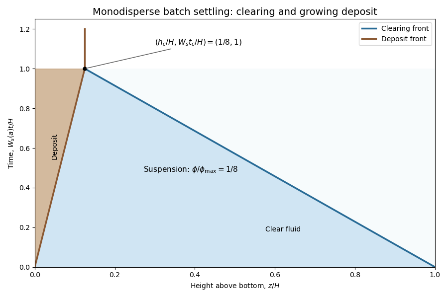
Codex 0 Created 2026-10-03 Updated 2026-10-14Use downward distance , with the height above the bottom, and write . This convention will also reproduce the printed negative deposit-front velocity in part (d). The ideal simple-cubic sphere packing has packing fraction ; leaving symbolic keeps the jump calculation independent of its value. In suspension, the kinematic sedimentation equation isIntegrate this conservation law across a moving discontinuity to obtain the Rankine-Hugoniot conditionThe brackets denote values on the increasing- side minus those on the other side. A sedimentation shock is a concentration jump moving at this secant slope of the particle flux. Deposited material is stationary and has zero flux.
For the upper clearing front, the states are and , giving downward. For the lower deposition front, the states are and , giving , upward. ThusIn terms of height above the bottom, the shock paths areThey meet when . Therefore complete settling occurs atThe final height also follows directly from particle volume fraction conservation, . The stationary deposit after the meeting carries no particle flux.
Past exam of the mathematics course of the University of Cambridge 2015 iii Paper 74 3 b Solution by Codex 0 Created 2026-10-03 Updated 2026-10-06
Codex 0 Created 2026-10-03 Updated 2026-10-06Let the particle and carrier-fluid mass densities be and , with identical density contrast for both species. At small particle Reynolds number, balance Stokes drag law against submerged weight:ConsequentlyAt large particle Reynolds number, use approximately constant drag coefficient and quadratic drag. Balancing against the same submerged weight gives , soBoth particles must lie in the constant- regime for this simple square-root ratio. More generally it contains an additional factor . The speeds are positive downward magnitudes; the signs of the shock velocities below depend on the chosen spatial coordinate.
Past exam of the mathematics course of the University of Cambridge 2015 iii Paper 74 3 a Solution by Codex 0 Created 2026-10-03 Updated 2026-10-06
Codex 0 Created 2026-10-03 Updated 2026-10-06A square circle packing of equal radii has one circle per cell of side . Its packing fraction is thereforeFor the alternating-radius square circle packing shown in the source figure, let be the nearest unlike-centre separation. A two-circle repeat cell has area and solid area . Unlike circles require ; like circles on the two sublattices require and . ThusAll three nonoverlap constraints matter when varying the radius ratio.
Take as in the illustrated arrangement and set . If , the large circles determine the spacing and increases with . If , unlike contacts determine it and , whose derivative is proportional to and is nonpositive. The maximum is therefore at the joining point:The large circles then touch their large neighbours, while each small circle exactly fills a square interstice. Interchanging the species gives the reciprocal radius ratio. This is the highest packing fraction within the specified alternating square arrangement; it is not a claim about every possible unequal-circle packing.
Past exam of the mathematics course of the University of Cambridge 2015 iii Paper 74 2 c Solution by Codex 0 Created 2026-10-03 Updated 2026-10-06
Codex 0 Created 2026-10-03 Updated 2026-10-06At the gravity current nose, the depth and velocity change over a distance comparable with the depth, with appreciable vertical acceleration and mixing. The hydrostatic approximation and the depth-uniform interior model do not resolve that structure. A suitable gravity-current front condition iswith a positive, order-one Froude number determined by the nose closure and geometry. It is not fixed by the interior equations alone. This definition uses ; if the front condition is expressed using , its numerical coefficient changes by .
For a late-time gravity-current box model, take the depth and particle volume fraction to be uniform over , and neglect entrainment and resuspension. The initial volume is , soThe total particle volume is . Deposition over the projected boundary width gives . With the specified hindered settling factor, the prismatic triangular-channel gravity-current box model isInitializing this approximate model with and matches the original volume and concentration; it does not assert that the immediate dam-break flow is a uniform box.
Eliminate time to obtainSince the left primitive is , the hindered-settling runout invariant in a prismatic triangular channel isThis relation, the volume constraint and determine the late-time evolution. If desired, the time is given by the quadrature . The physical branch has nonnegative right-hand side in the boxed relation; it ends when that expression reaches zero.
Thus the limiting runout length of a gravity current, measured from the closed end, isThe advance beyond the dam is . In the dilute limit, . The ideal model approaches its finite runout length of a gravity current only as : near the limit decays exponentially with rate and the front speed tends to zero. The exponent uses the prismatic triangular geometry; a channel widening with has a different volume constraint and runout law.
Past exam of the mathematics course of the University of Cambridge 2015 iii Paper 74 2 b Solution by Codex 0 Created 2026-10-03 Updated 2026-10-06
Codex 0 Created 2026-10-03 Updated 2026-10-06The channel is prismatic: its width depends on height, not on . A layer of depth has cross-sectional area . Volume conservation gives . With , the integrated excess hydrostatic pressure force isThus the streamwise momentum balance is . Under the specified vertical-settling approximation, the horizontal projection of the depositional boundary has width , so the particle balance is , where is the downward speed magnitude. The prismatic triangular-channel shallow water equations are thereforeThe pressure coefficient is the section-weighted mean of . The factor two in deposition comes from top width divided by area. There is no streamwise widening term, because is constant along the channel.
Define the positive characteristic speed scale . In variables the equations becomeThe coefficient matrix of this hyperbolic system has eigenvalues . Hence the three characteristic families areAlong , the concentration equation is the ordinary differential equation . Along , the left eigenvectors give the sedimenting triangular-channel characteristic compatibility equationsHere every derivative in a given equation follows that characteristic family, and . These three compatibility equations form the characteristic description; they are not three independent closed equations for all fields on any one curve. In particular, are not conserved Riemann invariants when the concentration varies: its differential and the deposition source must both be retained. The description assumes ; the dry or zero-buoyancy limit is degenerate.
Past exam of the mathematics course of the University of Cambridge 2015 iii Paper 74 2 a Solution by Codex 0 Created 2026-10-03 Updated 2026-10-06
Codex 0 Created 2026-10-03 Updated 2026-10-06The Boussinesq approximation requires . The reference mass density can then be used in inertia, while the small density excess is retained in buoyancy. Dilute particle volume fraction alone does not suffice if is exceptionally large. Define , so the reduced gravity is .
The shallow water equations require depth small compared with the horizontal evolution scale, weak vertical acceleration and approximately hydrostatic pressure. Here the ambient is deep and quiescent, so its leading contribution is a hydrostatic reference pressure; the excess pressure in the layer is . The model also needs nearly uniform streamwise velocity across the section and the stated absence of secondary circulation. The advancing gravity current nose is a separate region where these assumptions can fail.
A nearly uniform particle volume fraction can be maintained by turbulent mixing with eddy diffusivity , provided and the mixing time is short compared with horizontal advection and bulk evolution. Equivalently, keeps the bulk settling-induced gradient small. The particles should respond rapidly enough to follow the mixing motions. A thin boundary layer adjacent to the absorbing bed or walls need not be well mixed.
Uniform bulk concentration does not imply zero sedimentation. The relative downward particle velocity still supplies a particle deposition flux of approximately to an absorbing boundary. Mixing redistributes the remaining particles and maintains the bulk concentration profile while its overall level decreases; it need not suspend every particle indefinitely. Deposition requires negligible resuspension in the model.
Past exam of the mathematics course of the University of Cambridge 2015 iii Paper 74 1 c Solution by Codex 0 Created 2026-10-03 Updated 2026-10-14
Codex 0 Created 2026-10-03 Updated 2026-10-14Use the spatial internal-wave ray tracing model, with , and reflect the rays so that the frequency and tangential wave number are preserved. At a vertical wall the horizontal energy direction reverses; at a horizontal wall the vertical energy direction reverses. On the sloping wall the reflection depends on internal-wave slope criticality. The three-reflection orbit below encounters that wall at a height above , so the wall reverses the horizontal energy direction there.
First take the packet to leave the bottom upward and to the left, with . The four segments of the loop areThe left-wall reflection is at and the top reflection at . The slope intersection solves , giving the internal-wave ray return mapThus the next formal bottom reflection is at . On , the slope heights are between approximately and , consistent with the assumed reflection type.
An internal-wave attractor is a stable periodic ray, so solve . This gives , and thereforeThe successive vertices areThis is clockwise circulation in the plane. Differentiating the internal-wave ray return map showsNeighbouring bottom intersections converge to the periodic orbit, geometrically focusing the energy beam.
For completeness, the opposite upward launch direction has the reversed three-reflection itinerary: slope, top, left. In the interval where this itinerary is valid, putThe three-reflection reverse map is , with domain . Its fixed point is the same, but . Counterclockwise packets defocus from that orbit. Except for the exactly periodic reverse ray, they eventually leave this itinerary. In the full geometric reflection construction, omitted-side or additional-slope reflections redirect generic rays into the clockwise attracting branch. Tangency and exactly critical reflections are singular exceptions requiring finite-wavelength or dissipative treatment.

Clockwise spatial internal-wave attractor and convergence of neighbouring ray loops in the trapezoidal basin
. Details. The bottom reflection is a formal spatial-ray idealization: part (b) shows that the WKB approximation itself fails near , so the diagram does not imply arrival and reflection there in finite WKB travel time. In a real fluid, viscous attenuation of an internal-wave beam, finite wavelength, internal-wave breaking and ensuing turbulence and mixing limit the beam width and energy density. Unlimited focusing is a property of the ideal geometric model, not a prediction for the resolved physical wave.
Past exam of the mathematics course of the University of Cambridge 2015 iii Paper 74 1 b Solution by Codex 0 Created 2026-10-03 Updated 2026-10-06
Codex 0 Created 2026-10-03 Updated 2026-10-06For a two-dimensional internal gravity wave with fixed horizontal wave number , the vertical velocity amplitude satisfiesThis follows from the Linearized Boussinesq equations just as in part (a), allowing the background buoyancy frequency to vary. The WKB approximation gives locallyIt requires slowly varying stratification compared with the local vertical wavelength, in particular , and a small-amplitude wave in the inviscid, nonrotating regime. Propagation requires ; where , the local vertical wave number is imaginary and the solution is evanescent. Turning levels and abrupt changes need a separate connection calculation. Finite viscosity, background flow, rotation or nonlinear effects require modifications of this model.
The ray tracing equations use the local dispersion relation as a Hamiltonian:The stationary, horizontally uniform background conserves the frequency and horizontal wave number. In two dimensions the group velocity gives . For the specified buoyancy frequency and , . Hence for the two geometric internal-wave rays through the specified point areEach curve has both directed propagation senses, giving four local directed rays. Their formal intersections with are and .
At , and : this is a double-zero internal-wave turning level, since touches zero without changing sign. The ray becomes vertical geometrically, but its group velocity tends to zero. Taking without loss of generality, the downward branch hasThe formal travel time diverges logarithmically as . Meanwhile grows, so the WKB approximation fails before that limit; its predicted amplitude cannot be extrapolated to infinity. The spatial ray reaches a finite limiting position, but finite-wavelength behaviour near the zero must be found beyond WKB. There is no evanescent half-space supplied by this particular , so ordinary simple-turning-point reflection cannot be assumed solely from the local ray construction.
Past exam of the mathematics course of the University of Cambridge 2015 iii Paper 74 1 a Solution by Codex 0 Created 2026-10-03 Updated 2026-10-06
Codex 0 Created 2026-10-03 Updated 2026-10-06Use the inviscid, nonrotating Boussinesq approximation, with a stable background mass density and reference density . Write for the perturbation buoyancy and for the kinematic pressure. The buoyancy frequency is . Dropping products of perturbations in the Boussinesq equations gives the Linearized Boussinesq equationsThe last equation expresses incompressible flow; the second follows by advecting the background mass density gradient. Neglecting rotation and viscosity is part of this internal gravity wave model.
For a plane internal gravity wave proportional to , put and . Eliminating the horizontal velocity, pressure and buoyancy from the linear equations givesFor example, the horizontal momentum and continuity equations give ; substituting into vertical momentum yields the displayed dispersion relation. Thus an IGW has in this model.
On the positive-frequency branch, the phase velocity normal to a constant-phase plane and the group velocity areConsequently , and phase and group velocity are perpendicular. Equivalently, the dispersion relation is homogeneous of degree zero in the wave vector, so differentiating with respect to its scale proves the same orthogonality. Energy travels with the group velocity, along the phase planes. At the degenerate limit , and the group velocity vanishes; the orthogonality statement then has this limiting interpretation.
Past exam of the mathematics course of the University of Cambridge 2015 iii Paper 73 1 c Solution by Codex 0 Created 2026-10-03 Updated 2026-10-06
Codex 0 Created 2026-10-03 Updated 2026-10-06The mobility correction from a fixed distant sphere givesTaking their ratio and keeping the first nonzero transverse correction yieldsto the stated leading order. Set . The deflection is , so replacing by on the right introduces only higher-order errors. Integrating from givesThe maximum occurs at , and the deflection and spin in a distant sphere encounter areFor the rotation, use and to leading order in the angular velocity from part (b). Its signed angle about the positive axis isThus the rotation is clockwise when viewed from positive , with the magnitude of the displayed leading term.
The deflection tends back to zero downstream: . More generally, kinematic reversibility of Stokes flow combined with reflection in the plane makes a passing trajectory fore-aft symmetric. One can see this without using the distant-sphere approximation: the relevant translational hydrodynamic mobility matrix has the form . Hence is even in and is odd in . Uniqueness of the trajectory through then gives .
For , the numerical deflection and spin approximations above are invalid: the encounter enters a narrow gap and requires lubrication theory. However, the same return to the incoming offset holds for an ideal passing encounter of perfectly smooth spheres in Stokes flow. Lubrication resistance prevents finite-time contact under a bounded force, and does not itself destroy kinematic reversibility of Stokes flow. Contact, surface roughness or nonhydrodynamic forces could change that conclusion; they are additional physics, not part of the ideal model. This distinction is the fore-aft symmetry of a sedimenting-sphere encounter.
Past exam of the mathematics course of the University of Cambridge 2015 iii Paper 73 1 b Solution by Codex 0 Created 2026-10-03 Updated 2026-10-06
Codex 0 Created 2026-10-03 Updated 2026-10-06Let , , and letUse the method of reflections for Stokes flow. At the fixed sphere, the first sphere produces the incident Stokeslet velocity to leading order. In Faxén translation law, set the second sphere's translational velocity to zero. The applied holding force is thereforeThe first sphere's finite-radius potential dipole adds to the incident velocity, as does the Laplacian term in Faxén translation law at the fixed sphere. Multiplying by gives the stated next correction. There is no intermediate term. This is the holding force and torque for a sphere in a distant Stokeslet.
The vorticity of a Stokeslet at displacement is . At the fixed sphere, , soSet its angular velocity to zero in Faxén rotation law. The applied holding couple isThe displayed sign is the external couple needed to oppose the ambient rotation, rather than the hydrodynamic couple on the sphere.
The leading reflected flow at the first sphere is . Apply Faxén translation law there with its prescribed force . Since , the mobility correction from a fixed distant sphere isThe next correction comes from finite-radius terms in the incident/reflected flow and in Faxén translation law, together with the fixed sphere's induced stresslet and holding-couple rotlet. Each gives at the first sphere. The symbol is its isolated-sphere velocity scale, not its actual velocity in the two-sphere problem.
The first sphere has no applied couple. Its angular velocity follows from Faxén rotation law and the reflected Stokeslet:The component of parallel to contributes no vorticity. The next reflected rotlet and stresslet give the stated error order.
Past exam of the mathematics course of the University of Cambridge 2015 iii Paper 73 1 a Solution by Codex 0 Created 2026-10-03 Updated 2026-10-06
Codex 0 Created 2026-10-03 Updated 2026-10-06One convention for the Papkovich–Neuber representation uses a harmonic vector potential and a harmonic scalar potential :These are harmonic functions away from any singular force point. Since , the representation gives and , the equations of homogeneous Stokes flow.
Place the point force at the origin. A velocity linear in , decaying as and having the rotational symmetry of a point force is obtained from , . The vector components are harmonic functions for ; scalar dipole potentials would instead generate higher-order decaying singularities. The force normalization fixes . Indeed, substitution gives the Stokeslet:To verify its strength, the Newtonian fluid stress tensor is . Its outward traction integrated over any sphere surrounding the origin is , because . Thus the localized force applied to the fluid is , as required. Translation of the origin gives the same Stokeslet centered at any prescribed force point.
Past exam of the mathematics course of the University of Cambridge 2015 iii Paper 72 2 b Solution by Codex 0 Created 2026-10-03 Updated 2026-10-06
Codex 0 Created 2026-10-03 Updated 2026-10-06Let be the stationary point and let be its real symmetric Hessian matrix. First suppose the stationary point is interior and nondegenerate, the oscillatory integral amplitude and oscillatory integral phase are sufficiently smooth, and boundary contributions are absent or smaller than the stationary contribution. Diagonalize by an orthogonal change of coordinates, with eigenvalues . Locally,Scaling each principal coordinate by and evaluating its Fresnel integral gives the two-dimensional stationary-phase formula:Here is the number of positive eigenvalues minus the number of negative ones: , or . The formula gives the leading nonzero term when . A partition of unity isolates this neighbourhood; integration by parts away from stationary points makes the remaining interior contribution smaller. For a smooth compactly supported oscillatory integral amplitude the local error is .
The printed assumption of a single stationary point alone is insufficient for an unconditional answer. A degenerate oscillatory integral phase with a smooth oscillatory integral amplitude supported near the origin has only one stationary point, but scales as . Boundary terms can also contribute at order : on the unit disk with oscillatory integral amplitude one and ,whose stationary contribution is and whose boundary contribution is . Thus the boxed formula is the standard nondegenerate interior stationary contribution, with the stated hypotheses; the data as printed do not determine all possible leading behaviours.
Past exam of the mathematics course of the University of Cambridge 2015 iii Paper 72 1 c Solution by Codex 0 Created 2026-10-03 Updated 2026-10-06
Codex 0 Created 2026-10-03 Updated 2026-10-06The stationary points of the exponent are and , because . The first is a local maximum with and ; the second is a local minimum. Alsoso the endpoint overtakes the interior maximum only when .
For fixed , the upper endpoint is the unique maximum. Linearizing the exponent there gives the Laplace endpoint estimate . At , only half of the local Gaussian integral is included. For , the whole Gaussian near contributes. At an endpoint has the same exponential height, but its prefactor is , smaller than the interior prefactor. For , the endpoint has strictly greater height and dominates.
Consequently all fixed- regimes areThe estimate follows from Laplace's method; the tail toward negative infinity is exponentially harmless since the cubic tends to negative infinity.
Pinned article: Introduction to the OurBigBook Project
Welcome to the OurBigBook Project! Our goal is to create the perfect publishing platform for STEM subjects, and get university-level students to write the best free STEM tutorials ever.
Everyone is welcome to create an account and play with the site: ourbigbook.com/go/register. We belive that students themselves can write amazing tutorials, but teachers are welcome too. You can write about anything you want, it doesn't have to be STEM or even educational. Silly test content is very welcome and you won't be penalized in any way. Just keep it legal!
Intro to OurBigBook
. Source. We have two killer features:
- topics: topics group articles by different users with the same title, e.g. here is the topic for the "Fundamental Theorem of Calculus" ourbigbook.com/go/topic/fundamental-theorem-of-calculusArticles of different users are sorted by upvote within each article page. This feature is a bit like:
- a Wikipedia where each user can have their own version of each article
- a Q&A website like Stack Overflow, where multiple people can give their views on a given topic, and the best ones are sorted by upvote. Except you don't need to wait for someone to ask first, and any topic goes, no matter how narrow or broad
This feature makes it possible for readers to find better explanations of any topic created by other writers. And it allows writers to create an explanation in a place that readers might actually find it.
Figure 1. Screenshot of the "Derivative" topic page. View it live at: ourbigbook.com/go/topic/derivativeVideo 2. OurBigBook Web topics demo. Source. - local editing: you can store all your personal knowledge base content locally in a plaintext markup format that can be edited locally and published either:This way you can be sure that even if OurBigBook.com were to go down one day (which we have no plans to do as it is quite cheap to host!), your content will still be perfectly readable as a static site.
- to OurBigBook.com to get awesome multi-user features like topics and likes
- as HTML files to a static website, which you can host yourself for free on many external providers like GitHub Pages, and remain in full control

Figure 2. You can publish local OurBigBook lightweight markup files to either OurBigBook.com or as a static website.
Figure 3. Visual Studio Code extension installation.
Figure 5. . You can also edit articles on the Web editor without installing anything locally. Video 3. Edit locally and publish demo. Source. This shows editing OurBigBook Markup and publishing it using the Visual Studio Code extension. 
- Infinitely deep tables of contents:




All our software is open source and hosted at: github.com/ourbigbook/ourbigbook
Further documentation can be found at: docs.ourbigbook.com
Feel free to reach our to us for any help or suggestions: docs.ourbigbook.com/#contact