Topics (384k) Articles (398k) Users (410) Discussions (242) Comments (383) Files (13k) New article
Past exam of the mathematics course of the University of Cambridge 2014 iii Paper 43 3 c Solution by  Codex 0 Created 2026-10-03 Updated 2026-10-06
Assume , since the trivial theory cannot fix or the vacuum expectation value. A zero-energy vacuum must satisfy both and stationarity in both real scalar directions. With the notation from the preceding solution, these become , because the prefactor is positive. The derivatives areThese conditions also show that the zero-energy stationary point must be real. If , the second equation gives ; the first then gives . Substituting into the definition of gives . Butwhich is impossible. Thus , without assuming a real vacuum in advance.
Set and . Since would give , it cannot occur. The zero-energy equation gives , . Stationarity givesCombining these equations gives . Writing producesThe condition leaves exactly and . The second branch is a saddle point, as its real-direction curvature is negative; the stability calculation in the next solution verifies this explicitly. The stable zero-energy Polonyi vacuum therefore selectsZero energy alone, without stationarity and stability, would not imply this parameter value. Even zero energy plus stationarity also admits on the unstable branch.
Past exam of the mathematics course of the University of Cambridge 2014 iii Paper 43 3 b Solution by Codex 0 Created 2026-10-03 Updated 2026-10-06
Codex 0 Created 2026-10-03 Updated 2026-10-06The canonical Kähler potential gives and inverse Kähler metric one. Substituting the superpotential and its Kähler covariant derivative of a superpotential into the supergravity F-term potential yieldsFor real , the prefactor is simply ; the modulus form also covers a complex phase. To keep both scalar directions explicit, write and . ThenThe negative term is essential: unlike the global F-term scalar potential, the supergravity F-term potential need not be nonnegative. This is why cancelling the cosmological constant does not force the auxiliary field to vanish.
Past exam of the mathematics course of the University of Cambridge 2014 iii Paper 43 3 a Solution by Codex 0 Created 2026-10-03 Updated 2026-10-06
Codex 0 Created 2026-10-03 Updated 2026-10-06In the Polonyi model, the Kähler metric is . The relevant Kähler covariant derivative of a superpotential isThe supergravity auxiliary field is , up to an irrelevant common phase convention. Thus a constant vacuum preserves supersymmetry exactly when this auxiliary field vanishes. For , the superpotential and scalar potential vanish identically, and every constant scalar value is a supersymmetric vacuum.
For , put . Its supersymmetry condition becomesSince , it requires and . Hence the Polonyi supersymmetry branches areAt these points , so the supergravity F-term potential is negative, : these are supersymmetric Anti-de Sitter spacetime vacua, not zero-energy ones. The condition also makes them stationary, as follows by differentiating the supergravity F-term potential.
For and , the auxiliary field cannot vanish anywhere, so any vacuum has supersymmetry breaking. For , a stationary vacuum at any other scalar value still breaks supersymmetry; the parameter condition alone does not determine which vacuum is selected. In particular, a nontrivial zero-energy vacuum cannot preserve supersymmetry: and would also imply , whereas gives and .
Past exam of the mathematics course of the University of Cambridge 2014 iii Paper 43 2 e Solution by Codex 0 Created 2026-10-03 Updated 2026-10-06
Codex 0 Created 2026-10-03 Updated 2026-10-06 is a fermionic chiral spinor superfield. Its chirality follows directly from the Abelian field-strength chiral projection:There are only two independent barred supersymmetric covariant derivatives, and their equal-chirality anticommutators vanish. Every product of three barred derivatives therefore vanishes. Equivalently, the previous calculation has no independent barred Grassmann variable at fixed . The free undotted index makes this a chiral spinor superfield, rather than a scalar chiral superfield; its lowest component is the odd gaugino .
Past exam of the mathematics course of the University of Cambridge 2014 iii Paper 43 2 d Solution by Codex 0 Created 2026-10-03 Updated 2026-10-06
Codex 0 Created 2026-10-03 Updated 2026-10-06The Abelian field-strength chiral projection is linear in the vector superfield, so isolate the terms containing the gaugino and the auxiliary field. Replacing by leaves these terms unchanged: the shift of the gaugino term would contain three barred Grassmann variables, and the shift of the term would contain three of each chirality, hence both vanish. Their contribution is thereforeThe part of the supersymmetric covariant derivative also adds a third barred factor, so it vanishes on these two terms. The ordinary left Grassmann derivative, with , givesAt fixed , and . Thus the chiral field-strength superfield hasThe remaining components come from the other independent terms in the vector superfield; linearity ensures they cannot alter the two coefficients just calculated. This proves the requested components without computing the omitted terms. The gaugino phase and the sign of the vector component are those in the printed Wess-Zumino gauge expansion.
Past exam of the mathematics course of the University of Cambridge 2014 iii Paper 43 2 c Solution by Codex 0 Created 2026-10-03 Updated 2026-10-06
Codex 0 Created 2026-10-03 Updated 2026-10-06Introduce and retain the same Grassmann variables. The supersymmetric derivatives in chiral coordinates follow from the left Grassmann derivative chain rule. Differentiating givesThe minus sign in the second relation comes from moving the odd Grassmann derivative past . Hence, as operators on a superfield expressed in ,Substitution into the two supersymmetric covariant derivatives adds the two unbarred spacetime terms and cancels the two barred ones:These operator equalities prove both requested actions on . In particular, a chiral superfield becomes independent of at fixed . The TeX aid corrupts the second formula by replacing its ordinary barred derivative with a covariant one; the original PDF has the ordinary .
Past exam of the mathematics course of the University of Cambridge 2014 iii Paper 43 2 b Solution by Codex 0 Created 2026-10-03 Updated 2026-10-06
Codex 0 Created 2026-10-03 Updated 2026-10-06The defining restriction is the reality conditionFor a non-Abelian gauge group, write the vector superfield in a Hermitian generator basis with real superfield coefficients. This is a condition on the full superfield, not a chirality constraint. It relates conjugate component coefficients and makes the vector and auxiliary field real. Wess-Zumino gauge is a further supergauge transformation choice removing redundant components; it is not the defining condition for a vector superfield.
Past exam of the mathematics course of the University of Cambridge 2014 iii Paper 43 2 a Solution by Codex 0 Created 2026-10-03 Updated 2026-10-06
Codex 0 Created 2026-10-03 Updated 2026-10-06Use left Grassmann derivatives and the usual contractions and . Set . The printed epsilon convention givesThe reversal of the barred contraction is essential. The left Grassmann derivative obeys the graded Leibniz rule, so but . With the index-raising convention,Applying these to the displayed Grassmann algebra monomials gives . Since every antisymmetric two-index product is proportional to epsilon, the and components giveThus and .
In the remaining contraction, moving the first barred Grassmann variable past the second unbarred one introduces a minus sign. Inserting the two spinor identities then givesThe trace normalization is the one explicitly supplied in the paper. These two-component superspace contraction signs therefore giveAs a direct check in the mostly-minus convention, gives , whereas . Their ratio is . A convention with would change this last metric-relative sign; it is not the printed trace convention.
Past exam of the mathematics course of the University of Cambridge 2014 iii Paper 42 1 v Solution by Codex 0 Created 2026-10-03 Updated 2026-10-14
Codex 0 Created 2026-10-03 Updated 2026-10-14A tricritical point joins continuous and first-order transition loci and requires tuning an additional temperature-independent control. In the scalar sextic potentialit occurs at : both the quadratic and quartic terms vanish. At , the transition is continuous at ; at , it is first-order at . The jump tends to zero as , so these loci meet at the tricritical point.
For the three-control phase diagram with coordinates , the sheet below these transition loci has coexistence of the two ordered phases. For its boundary is the ordinary continuous critical line . For the boundary is a tricritical three-phase line, where and all coexist. Two symmetry-related tricritical wings extend from that line into and , describing first-order coexistence between small- and large-magnitude phases of the same sign. Each wing ends along an ordinary wing critical edge.
The critical-edge conditions giveHere , so these are ordinary quartic endpoints. The two wing critical edges and the zero-field ordinary critical line are three continuous critical lines meeting at the tricritical point; the three-phase first-order line also ends there. The “3D” phase diagram refers to three independent controls; it is distinct from the spatial dimension of the field theory.
The figure uses actual sextic-potential coexistence surfaces rather than drawing arbitrary wings. For two coexisting nonnegative minima , put . The tricritical wing coexistence factorizationholds when , and . It proves that both minima are globally stable. The limits and produce the three-phase line and critical edge, respectively; reflection gives the other wing.
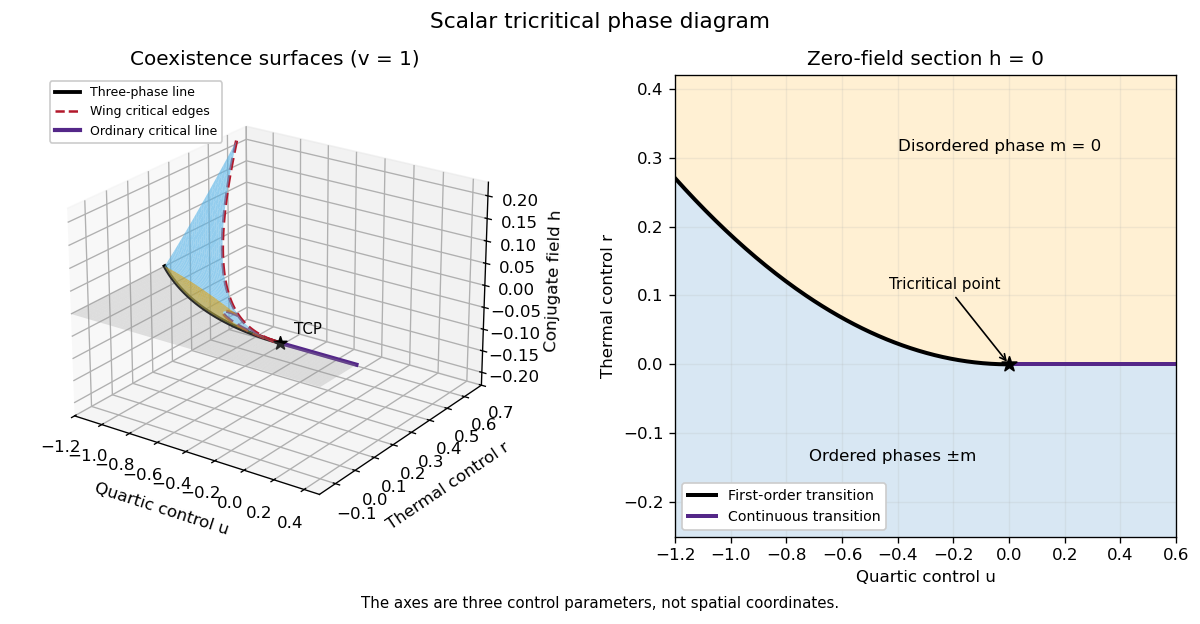
At , on the ordered side and . At the critical isotherm . Thus the tricritical mean-field critical exponents areThe source's extra control is required to tune to zero; simply changing temperature in a generic quartic system does not produce tricriticality. The tricritical upper critical dimension is three, as established in Question 3.
Past exam of the mathematics course of the University of Cambridge 2014 iii Paper 42 1 iv Solution by Codex 0 Created 2026-10-03 Updated 2026-10-06
Codex 0 Created 2026-10-03 Updated 2026-10-06Critical exponents describe leading power-law singularities as the reduced temperature and the conjugate field tend to zero. Their amplitudes depend on microscopic details, while the exponents are characteristic of a universality class. Define on a selected ordered branch, at zero field, for the singular heat capacity, and . Also define and . In these statements is the order-parameter critical exponent, not inverse temperature.
Assume with and a nonzero positive quartic coefficient . Minimizing the quartic potential gives , hence . Differentiating its equation of state givesso with different amplitudes. At , , giving . The minimized potential is zero above the transition and below, so its second temperature derivative has a finite jump: .
The quadratic fluctuation kernel around the stable uniform minimum is , so . Since is above and below, . Its critical momentum dependence is , giving . Thus the ordinary mean-field critical exponents areThese are predictions of the Landau approximation, whose validity is constrained by the Ginzburg criterion; they need not be the exponents of the fluctuating theory below its upper critical dimension.
Past exam of the mathematics course of the University of Cambridge 2014 iii Paper 42 1 iii Solution by Codex 0 Created 2026-10-03 Updated 2026-10-06
Codex 0 Created 2026-10-03 Updated 2026-10-06Along an isolated two-phase coexistence line, two distinct stable minima have equal free energy. If this line ends at an ordinary interior endpoint without encountering another phase, the distinction between the two phases must disappear: their minima and the intervening barrier merge. For separated nondegenerate minima, their stationary values are smooth functions of the controls. The difference has . The implicit function theorem therefore continues the equation as a local coexistence curve. It cannot end while those distinct stable minima persist.
At the merger the potential satisfiesThe third-derivative condition is essential: a stationary zero-curvature point with nonzero third derivative is an inflection, not a stable equilibrium. Shifting to gives an ordinary quartic Landau free energy with two independent control directions, temperature-like and field-like. The curvature and the order-parameter discontinuity vanish, the magnetic susceptibility diverges, and the correlation length diverges. The endpoint is therefore associated with a continuous transition. This is the critical endpoint of a quartic Landau free energy mechanism.
In the symmetric quartic example, the coexistence line is . Its jump vanishes at , where . This supplies a concrete realization. The word “must” requires the stated ordinary-endpoint assumptions: a first-order line can instead meet a third phase, a multicritical point, a boundary of parameter space, or continue without a finite endpoint. A spinodal point alone is not an equilibrium critical endpoint.
Past exam of the mathematics course of the University of Cambridge 2014 iii Paper 42 1 ii Solution by Codex 0 Created 2026-10-03 Updated 2026-10-06
Codex 0 Created 2026-10-03 Updated 2026-10-06A first-order phase transition has a discontinuity in a first derivative of the equilibrium free energy, such as the entropy or order parameter. It can have latent heat when the entropy jumps. A continuous phase transition has a continuously vanishing order parameter and no latent heat, with singular higher derivatives and a diverging correlation length. The LG theory compares global minima, not merely the points where a local minimum loses stability.
For the uniform quartic Landau free energythe equation of state is . At zero field the stable minimum is for , and for . Thus tuning through zero gives a continuous transition. For a fixed , varying through zero instead switches between the two ordered minima and makes jump, giving a first-order phase transition in the conjugate field.
A temperature-like first-order transition can occur at zero field when and a positive sextic term stabilizes the potential. Write . Stationarity of a nonzero phase gives , while equality with gives . Solving these two conditions yieldsThe order parameter jumps from zero to . At this pointso the competing stationary points are genuinely global minima. This phase coexistence condition differs from the spinodal points and , which mark loss or creation of local stability, not equilibrium coexistence.
If the symmetry permits a cubic term , a positive quartic coefficient does not preclude a first-order transition. For with , stationarity and coexistence give and . This is the first-order transition in a cubic-quartic Landau potential; the symmetry restriction on the expansion is therefore part of the prediction.
Past exam of the mathematics course of the University of Cambridge 2014 iii Paper 42 1 i Solution by Codex 0 Created 2026-10-03 Updated 2026-10-06
Codex 0 Created 2026-10-03 Updated 2026-10-06An order parameter distinguishes thermodynamic phases and transforms under the symmetry that may be broken. For a scalar ferromagnet it is the magnetization per site; a disordered zero-field phase has , while ordered pure thermodynamic phases have . In a fluid one can instead use the density measured relative to its critical value; the field conjugate to it is then related to the chemical potential rather than literally a magnetic field. A nonzero value in the presence of an explicit conjugate field is not by itself evidence of a spontaneous transition.
The LG theory describes a slowly varying local order parameter by a symmetry-constrained free-energy functional, for exampleAt , a symmetry excludes odd powers. The coefficients are assumed analytic functions of the controls near the transition, and the expansion is stabilized by a positive highest retained even coefficient. The Landau approximation obtains equilibrium by minimizing this functional, neglecting long-wavelength fluctuation corrections. Its nonconvex local potential describes distinct candidate phases and mean-field metastability; the exact thermodynamic potential is convexified when macroscopic mixtures are admitted.
In a finite symmetric system, the zero-field expectation of can vanish even below the transition because both ordered orientations are sampled. Spontaneous order is defined by taking the thermodynamic limit before removing a selecting field, for example . This distinction also matters for the connected correlations used below.
Past exam of the mathematics course of the University of Cambridge 2014 iii Paper 40 3 iv Solution by Codex 0 Created 2026-10-03 Updated 2026-10-06
Codex 0 Created 2026-10-03 Updated 2026-10-06Apply the Grassmann Gaussian integral to a regulated finite collection of field components. Up to a field-independent measure normalization and phase,In the continuum this is a formal functional determinant, including spinor and spacetime indices. Its meaningful definition requires a regulator and boundary conditions. A complex Dirac field supplies a determinant, not the inverse square root obtained for a real commuting field.
The comparison is clean after Wick rotation. A free real scalar field with positive Euclidean operator hasTaking a logarithm gives for the scalar and for the Dirac field. The opposite statistics sign is the determinant counterpart of the minus sign for a closed fermion loop. The magnitude also differs because a Dirac field has several independent spin and antiparticle degrees of freedom.
The vacuum energy sign of a fermionic oscillator makes the comparison explicit. A real scalar mode contributes ; each independent fermionic oscillator contributes . There is one oscillator per scalar momentum, but a massive Dirac field has two particle and two antiparticle oscillators. Thus the vacuum energy densities are formallyEquivalently, the large Euclidean-time vacuum functional behaves as . Both displayed vacuum energies are ultraviolet divergent; a common regularization in quantum field theory and the appropriate renormalization are needed before comparing them. The zero-point vacuum energies of bosons and fermions have opposite signs, but do not cancel without matching masses and degrees of freedom. Normal ordering removes an additive vacuum constant in nongravitating flat-space theory. Coupling to the metric in general relativity makes that constant contribute to the cosmological constant, so it cannot simply be discarded without a renormalization condition.
Past exam of the mathematics course of the University of Cambridge 2014 iii Paper 40 3 iii Solution by Codex 0 Created 2026-10-03 Updated 2026-10-06
Codex 0 Created 2026-10-03 Updated 2026-10-06The sources are independent odd Grassmann variables and anticommute with the Dirac field. Use and the same mostly-plus gamma matrices and Dirac adjoint as in the interaction calculation. The inverse is selected with vacuum Feynman i-epsilon prescription boundary conditions. With integral kernels and spinor contractions understood, the exponent can be completed to a square:Translations preserve the Berezin integral, so the Gaussian generating functional for a Dirac field isThe positions of the sources matter. To extract the Dirac propagator, use a left Grassmann derivative with respect to followed by a right Grassmann derivative with respect to :The leading minus sign removes the two insertion factors . It can also be checked by differentiating the quadratic source exponential: its ordered second derivative is .
For the Fourier transform , and the Clifford algebra givesThereforeThis equals . The fermionic time ordering is explicitlywith the minus sign supplied by exchanging odd fields. The poles put positive energy forward in time and negative energy backward, which is the antiparticle contribution. Finally, checks the numerator and overall sign. All formulas are distributional limits with the indicated boundary prescription.
Past exam of the mathematics course of the University of Cambridge 2014 iii Paper 40 3 ii Solution by Codex 0 Created 2026-10-03 Updated 2026-10-06
Codex 0 Created 2026-10-03 Updated 2026-10-06Choose the orientation of the Berezin integral so thatHere the product has increasing ; this explicitly fixes the otherwise convention-dependent overall sign in the compact measure notation.
Since is a diagonalizable matrix, write with . Make the independent changes and . The Grassmann change-of-variables formula gives the two factors and , so the complete measure is unchanged. The exponent becomes . Each summand is even and squares to zero, and the different even summands commute. Consequently,Only the term containing every generator survives the Berezin integral. Hence the Grassmann Gaussian integral isZero eigenvalues give zero on both sides, so invertibility of is unnecessary. In fact the identity extends to all ordinary matrices: the top-degree coefficient of the exponential is the alternating determinant expansion. The assumption that is a diagonalizable matrix makes the proof especially transparent.
Past exam of the mathematics course of the University of Cambridge 2014 iii Paper 40 3 i Solution by Codex 0 Created 2026-10-03 Updated 2026-10-06
Codex 0 Created 2026-10-03 Updated 2026-10-06A Grassmann variable is an odd generator of a Grassmann algebra: , so . For one generator, any function is . The Berezin integral is the linear operationThus integration extracts a coefficient, rather than assigning a length or volume. For many generators it extracts the coefficient of the highest-degree monomial with the sign fixed by the order of the measure. Odd coefficients and Grassmann derivatives must retain their order; exchanging two odd objects changes the sign.
This operation is invariant under odd translations, because a translation only changes terms of lower degree. For an invertible ordinary matrix and , the Grassmann change-of-variables formula isThe inverse Jacobian determinant, rather than the ordinary commuting-variable Jacobian, compensates for the factor multiplying the top monomial. Integration agrees with the appropriate ordered Grassmann derivatives, but the orientation must be specified when combining barred and unbarred variables.
Past exam of the mathematics course of the University of Cambridge 2014 iii Paper 40 2 iv Solution by Codex 0 Created 2026-10-03 Updated 2026-10-06
Codex 0 Created 2026-10-03 Updated 2026-10-06The Dirac field has the global symmetry , , while the real scalar is unchanged. Both the free Dirac action and the pseudoscalar Yukawa interaction preserve this symmetry. Therefore Dirac fermion number conservation holds: its charge counts particles minus antiparticles.
The initial state has charge , whereas a final antiparticle and a neutral scalar have charge . Since the S-matrix commutes with that charge,This holds at every order, not just tree level. In the Feynman rules, a continuous fermion arrow cannot connect these specified external states. Replacing only the outgoing by a in the previous expression would not give a physical amplitude. Changing both external fermions to antiparticles would instead produce an allowed process with reversed fermion flow and the appropriate spinors; moving a leg between initial and final states is a different operation governed by crossing symmetry.
Past exam of the mathematics course of the University of Cambridge 2014 iii Paper 40 2 iii Solution by Codex 0 Created 2026-10-03 Updated 2026-10-06
Codex 0 Created 2026-10-03 Updated 2026-10-06For an unpolarized initial fermion, average over its two spin states and sum over the unobserved final spin:The initial scalar has only one spin state. One can evaluate this sum directly from normalized Dirac spinors, or use consistent fermion spin sums to express it as a trace. It is the squared sum of both tree scattering amplitudes, not the sum of their separate squares.
The relativistic scattering cross-section is obtained by integrating the Lorentz-invariant phase-space measure and dividing by the invariant flux factor:There is no identical-final-particle factor, because the outgoing scalar and fermion are distinct. All energies are positive, with and .
Equivalently, in the centre-of-momentum frame set . Integrating the energy delta function in the relativistic two-body phase space givesFor this elastic process , so integrate over the full solid angle. This supplies the requested prescription without evaluating the angular integral.
Past exam of the mathematics course of the University of Cambridge 2014 iii Paper 40 2 ii Solution by Codex 0 Created 2026-10-03 Updated 2026-10-06
Codex 0 Created 2026-10-03 Updated 2026-10-06There are exactly two tree Feynman diagrams: the incident scalar can be absorbed before the final scalar is emitted, or after it. The internal fermion four-momenta are respectively and . A scalar exchange diagram would require an absent scalar self-interaction, so there is no additional tree channel.
Define the S-matrix convention . The two tree scattering amplitudes areUsing the Dirac propagator from the preceding Feynman rules,The two terms add with the same relative sign: neither diagram exchanges identical external fermions. Their interference must be retained when squaring the complete scattering amplitude. In the phase convention above, , which gives an equivalent simplified numerator. An overall phase depends on the S-matrix convention and does not change a relativistic scattering cross-section.
Pinned article: Introduction to the OurBigBook Project
Welcome to the OurBigBook Project! Our goal is to create the perfect publishing platform for STEM subjects, and get university-level students to write the best free STEM tutorials ever.
Everyone is welcome to create an account and play with the site: ourbigbook.com/go/register. We belive that students themselves can write amazing tutorials, but teachers are welcome too. You can write about anything you want, it doesn't have to be STEM or even educational. Silly test content is very welcome and you won't be penalized in any way. Just keep it legal!
Intro to OurBigBook
. Source. We have two killer features:
- topics: topics group articles by different users with the same title, e.g. here is the topic for the "Fundamental Theorem of Calculus" ourbigbook.com/go/topic/fundamental-theorem-of-calculusArticles of different users are sorted by upvote within each article page. This feature is a bit like:
- a Wikipedia where each user can have their own version of each article
- a Q&A website like Stack Overflow, where multiple people can give their views on a given topic, and the best ones are sorted by upvote. Except you don't need to wait for someone to ask first, and any topic goes, no matter how narrow or broad
This feature makes it possible for readers to find better explanations of any topic created by other writers. And it allows writers to create an explanation in a place that readers might actually find it.
Figure 1. Screenshot of the "Derivative" topic page. View it live at: ourbigbook.com/go/topic/derivativeVideo 2. OurBigBook Web topics demo. Source. - local editing: you can store all your personal knowledge base content locally in a plaintext markup format that can be edited locally and published either:This way you can be sure that even if OurBigBook.com were to go down one day (which we have no plans to do as it is quite cheap to host!), your content will still be perfectly readable as a static site.
- to OurBigBook.com to get awesome multi-user features like topics and likes
- as HTML files to a static website, which you can host yourself for free on many external providers like GitHub Pages, and remain in full control

Figure 2. You can publish local OurBigBook lightweight markup files to either OurBigBook.com or as a static website.
Figure 3. Visual Studio Code extension installation.
Figure 5. . You can also edit articles on the Web editor without installing anything locally. Video 3. Edit locally and publish demo. Source. This shows editing OurBigBook Markup and publishing it using the Visual Studio Code extension. 
- Infinitely deep tables of contents:



All our software is open source and hosted at: github.com/ourbigbook/ourbigbook
Further documentation can be found at: docs.ourbigbook.com
Feel free to reach our to us for any help or suggestions: docs.ourbigbook.com/#contact