The quadratic polynomial $x^2+4x+10=(x+2{)}^2+6$ has no real roots of a polynomial. Thus the characteristic polynomial does not split over the real numbers. A real diagonal matrix would have only real eigenvalues, and similar matrices have the same characteristic polynomial. Therefore $A$ is not diagonalizable over $\mathbb{R}$.

Over the complex numbers, the three eigenvalues areThey are distinct. Each is a root of the minimal polynomial, so here the minimal polynomial equals the characteristic polynomial and has distinct linear polynomials. Consequently $A$ is diagonalizable over $\mathbb{C}$.

No. On any nonzero vector space over a field of characteristic two, take $E=F=I$. Both are linear projections, andThe correct condition from part (i) in this characteristic is $EF=FE$, because minus and plus coincide. Vanishing of both products remains sufficient, but is no longer necessary.

Suppose first that $E+F$ is a linear projection. Part (i) gives $EF=-FE$. Multiplying on the left by $E$ gives $EF=-EFE$, and multiplying on the right by $E$ gives $EFE=-FE=EF$. Combining them yieldsIn a field of characteristic different from two, the nonzero scalar $2$ is invertible. Hence $EF=0$, and $FE=-EF=0$ too. Conversely these two zero products make the expansion in part (i) equal zero. ThereforeThe argument cancels a nonzero scalar, never a possibly singular linear map.

Expand the square using $E^2=E$ and $F^2=F$:ThusThis sum of two linear projections criterion holds in every characteristic; it uses an equality of linear maps, not cancellation of factors in the noncommutative associative algebra of linear endomorphisms.

The same invariant subspaces work for $S=\alpha I+\beta T$: it acts by $\alpha$ on $\ker T$ and by $\alpha +\beta$ on $\mathrm{im}T$. Its minimal polynomial is therefore the product of the distinct linear polynomials belonging to the nonzero summands. Explicitly,When $\beta \ne 0$, the two candidate eigenvalues are distinct in any field. This is the minimal polynomial of an affine function of a projection.

Put $n=\dim V>0$ and $r=\mathrm{rank}T$. The direct sum in part (i) givesThe eigenvalues are the members of $\{0,1\}$ actually present: zero occurs exactly when $r<n$, and one exactly when $r>0$. Since $T$ is diagonalizable, its minimal polynomial contains each present eigenvalue once:In particular, a nonzero vector space does not force both eigenvalues to occur. The zero and identity maps are important special cases.

The identity $T^2=T$ gives the decompositionThe first summand lies in the kernel of a linear map $\ker T$, and the second in the image of a linear map $\mathrm{im}T$. If $w$ belongs to their intersection, write $w=Tu$; then $Tw=T^{2}u=Tu=w$, while $Tw=0$. Thus $w=0$, proving the direct sumOn these two invariant subspaces, $T$ is respectively zero and the identity map. Joining a basis of each produces a basis of eigenvectors, with matrixHence every linear projection is diagonalizable, over the original field, including in characteristic two.

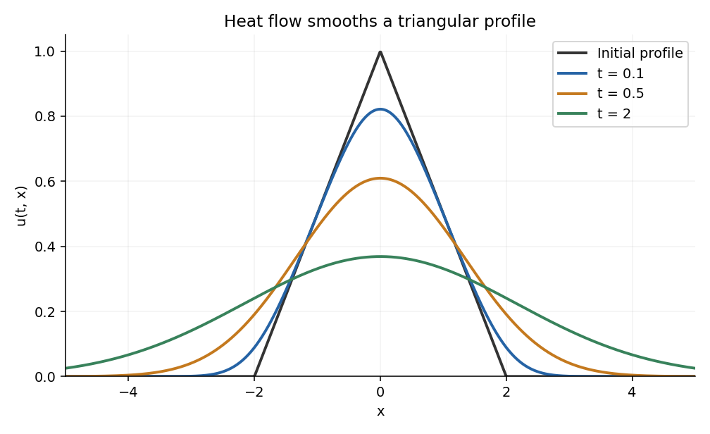
Insert part (i) in the inverse Fourier transform. The factor two in $\hat{T}$ cancels half of the inverse normalization:The integrand has a removable singularity at zero. For $t>0$, the Gaussian controls every polynomial factor at infinity, so differentiation under the integral is valid. Differentiation in $t$ and twice in $x$ both multiply the integrand by $-{\omega }^2$, proving $u_t=u_{xx}$.

There is also a direct physical-space representation:Since $q_t$ has integral one, writeThe continuous compactly supported profile $T$ is uniformly continuous. Given $ϵ>0$, choose $\delta >0$ so its change is below $ϵ$ for $|y|<\delta$. That part of the integral is bounded by $ϵ$. The other part is bounded by $2\Vert T{\Vert }_{\infty }{\int }_{|y|\ge \delta }{q}_t(y)dy$, which tends to zero by the substitution $y=2\sqrt{t}z$ and the vanishing tails of the Gaussian integral. This proves $u(t,x)\to T(x)$ uniformly as $t\downarrow 0$ and verifies the initial condition.

Thus the formula supplies the full heat evolution of a triangular profile, including the corner points of the initial profile. Positive time immediately smooths those corners.

For fixed frequency $\omega$, the Fourier transform of a derivative gives $\widehat{u_{xx}}=-{\omega }^2\hat{u}$. The transformed initial value problem is thereforeSolving this scalar ordinary differential equation yieldswhere the value at $\omega =0$ is interpreted by continuity and equals two. Thus diffusion suppresses high frequencies by the Gaussian multiplier while preserving the zero-frequency mass.

The differentiation and transform steps are justified for the heat kernel solution $u=q_t\ast T$: for positive time its spatial derivatives are integrable, since Gaussian derivatives are integrable and $T$ is bounded with compact support. Alternatively, the transformed calculation first suggests the formula, and the next part verifies the resulting solution directly.

Use an exponential perturbation whose image under $L$ is strictly positive everywhere. The coefficient $r$ is bounded on the closed disk; put $R={\max }_{\overline{D}}|r|$ and choose $k>R$, $k>0$. For $v(x,y)=e^{kx}$,Consequently $u_{ϵ}=u+ϵv$ satisfies $L{u}_{ϵ}=f+ϵLv>0$. Part (i) applies, so for every $z\in \overline{D}$,Letting $ϵ\downarrow 0$ givesThus the maximum is attained on the boundary also when $f\ge 0$. This is the exponential perturbation proof of the weak maximum principle with drift. It does not require differentiating the continuous coefficients $r,s$.

Write the elliptic differential operator as $L=\Delta +r{\partial }_x+s{\partial }_y$. At an interior maximum, $u_x=u_y=0$ and $u_{xx}+u_{yy}\le 0$. Therefore $Lu\le 0$ there, contradicting $Lu=f>0$.

The extreme value theorem ensures that a maximum exists on the compact closed disk. It cannot lie in the interior, so the maximum is attained on $\partial D$. The drift terms disappear at a stationary point, which is why the strict-sign proof is so short.

For every $a\ne 0$ and every real $b$, there is exactly one solution on the maximal connected interval containing $a$. The formula in part (i) proves existence on the entire appropriate half-line, and the initial condition fixes its sole constant uniquely. This agrees with the local Picard-Lindelöf theorem.

For $a=0$, there is no classical solution on an interval containing the initial point, whatever $b$ is: the printed equation is not defined there. Even if one only imposes the equation for $x\ne 0$ and asks for a finite continuous extension across zero, the negative side rules it out. For $x\to 0^{-}$:

Thus no choice of the negative-side integration constant admits a finite left limit.

There is a useful distinction with a separately extended one-sided problem. On $x>0$, every member of the solution family tends to zero with all its derivatives as $x\downarrow 0$, since the exponential dominates every inverse power of $x$. If the forcing is separately defined to be zero at the right endpoint, that modified one-sided problem has infinitely many smooth solutions with $y(0)=0$, and none with $y(0)\ne 0$. Those one-sided extensions do not give solutions on the two-sided intervals in the question.

On either connected half-line, the homogeneous linear differential equation isIntegration gives $\boxed{y_h=C{x}^{-2}{e}^{-1/x}}$, including the zero solution. For the inhomogeneous equation choose the positive integrating factorIt satisfies ${\mu }^{\prime }/\mu =2/x-1/x^2$. Multiplication gives the exact derivativeHence all solutions on either half-line areFor $a\ne 0$, impose $y(a)=b$ to obtain $C=a^2{e}^{1/a}b-\arctan a$. The complete initial value problem solution is thereforeIt is smooth throughout the maximal connected interval $(0,\infty )$ if $a>0$, and $(-\infty ,0)$ if $a<0$.

Take any $a\ne 0$ and any $b\in \mathbb{R}$. Choose $0<h_0<|a|$, so $[a-h_0,a+h_0]$ avoids zero. Onboth $f$ and $f_y=(1-2x)/x^2$ are continuous. They are bounded by compactness, and the bound on $f_y$ gives the uniform Lipschitz continuity in $y$ required by the Picard-Lindelöf theorem.

If $M$ is a bound for $|f|$, shrink $h$ so $0<h<h_0$ and $hM<1$. Then the solution has $|y(x)-b|\le hM<1$, which supplies even strict inequalities at both edges of the requested vertical strip.

At $a=0$, neither $f$ nor the original exponential expression is defined. Thus the theorem applies exactly for $a\ne 0$, with no restriction on $b$. Failure of the hypotheses alone would not prove nonexistence; the explicit solutions below settle that issue.

For fixed $a\ne 0$ and $B>0$, the rectangleis compact and stays away from $x=0$. The function $f$ in part (i) is continuous there. The extreme value theorem makes $|f|$ attain a finite maximum $M_0$ on $K$; choosing $\boxed{M=M_0+1}$ gives the requested strict bound.

The absolute values make this a positive-$x$ rectangle even when $a<0$. Its boundedness is still true, but for a negative initial point the Picard-Lindelöf theorem must instead be applied to a rectangle centered at that negative point, as in part (iii).

Dividing by $x^2$, which is allowed precisely away from zero, givesThis function is smooth on each of the two half-planes $x>0$ and $x<0$, and is affine in the dependent variable $y$. Its derivative with respect to $y$ is $(1-2x)/x^2$.

Work inside $V_{m+1}$, and take the orthogonal complement for a bilinear form of $U=V_m$ relative to this ambient space. If $z\in U\cap U^{\perp }$, then $\phi (z,z)=0$, so positive definiteness on $U$ forces $z=0$.

Part (a)(iv) therefore gives $V_{m+1}=U\oplus U^{\perp }$, with $\dim U^{\perp }=1$. Choose $w\ne 0$ spanning that complement and use the basis $e_1,\dots ,e_m,w$. Symmetry and orthogonality make its Gram matrixBy part (b)(i), $\det B=(\det P{)}^2\det A_{m+1}>0$. Part (ii) applied to the already positive definite restriction gives $\det A_m>0$. ThereforeFor a nonzero vector $u+tw$ with $u\in U$,This proves positive definiteness on $V_{m+1}$.

Finally $\det A_1>0$ says $\phi (e_1,e_1)>0$, so the restriction to $V_1$ is positive definite. Induction using all successive positive leading principal minors reaches $V_n=V$. Combined with part (ii), this proves Sylvester's criterion in both directions.

The restriction of a positive definite form to each $V_m$ is positive definite. By the spectral theorem for real symmetric matrices, choose an orthogonal matrix $P$ such that $P^T{A}_{m}P=\mathrm{diag}(d_1,\dots ,d_m)$.

Each $d_i=\phi (f_i,f_i)>0$, since a basis vector is nonzero. Taking determinants in part (i) givesbecause an orthogonal matrix has determinant $\pm 1$. ConsequentlyThese determinants are the leading principal minors in Sylvester's criterion.

Use the $m$-dimensional space $V_m$ for this change of basis. With the columns of $P$ recording the new basis in the old one, bilinearity givesThus the matrices of the bilinear form satisfyThis is matrix congruence, rather than the similarity rule for an endomorphism: both arguments of the bilinear form change basis.