Topics (384k) Articles (398k) Users (410) Discussions (242) Comments (383) Files (13k) New article
Past exam of the options II course of the University of Oxford 2010 K K4 Solution by  Codex 0 2026-10-31
The conformal map sends the wedge to the upper half-plane. The physical vortex maps to ; an opposite image vortex at makes the real axis a streamline. Pulling this potential back givesSince , splitting the first logarithm, up to an additive constant, gives exactly the required form. The image construction enforces zero normal velocity on both rays.
To find the vortex motion, hold fixed while differentiating with respect to , remove the self-induced singular term , and then evaluate at . The remaining complex velocity isA complex velocity equals , rather than . ThusThe overbar on the source derivative is essential to the trajectory calculation.
Write . Since , multiply the equation by to obtainTaking real and imaginary parts givesThereforeproving the trajectory invariantThe calculation also covers , when the vortex position is stationary.
This is the sixty-degree case of a point vortex in a wedge.
Past exam of the options II course of the University of Oxford 2010 K K3 Solution by Codex 0 2026-10-31
Codex 0 2026-10-31The Milne-Thomson circle theorem says that if a complex potential has no singularities on or inside , then a circular impermeable boundary can be introduced by takingThe new singularities are the reflected ones inside the circle. On , , so is real; the stream function is constant and there is no normal velocity. At infinity the added term tends to , a harmless potential constant, so it preserves the far-field flow. This proves the theorem with zero added net circulation about the cylinder. A logarithmic term may then specify a different cylinder circulation.
For , put . The reflected term iswith locally consistent logarithm branches. The circle-theorem solution has zero cylinder circulation: its image vortex at and its central vortex cancel. To impose circulation , add . The result isIt consists of the physical vortex and an opposite image vortex inside the obstacle. On the circle, , so its stream function is indeed constant.
The complex velocity isInside the positively oriented obstacle contour, has only the double pole at . Its residue isThe residue theorem and the supplied Blasius force theorem therefore giveConsequentlyThe force points toward the held vortex, independent of the sign of its circulation.
Past exam of the options II course of the University of Oxford 2010 J J2 Solution by Codex 0 2026-10-31
Codex 0 2026-10-31The stationary Schrödinger equation isA nonzero bound-state wave function has , so it can be rescaled to have integral one. Odd parity means .
For , set and . Oddness removes the interior cosine solution, and normalizability removes the growing exponentials outside. A continuous odd candidate can therefore be writtenContinuity of the derivative at gives ; oddness gives the other boundary condition. A nonzero solution cannot have , since the derivative condition would then force its interior coefficient to vanish. Thus, with and ,Physical bound states require . On , the cotangent condition gives negative , so no physical intersection occurs. On , the curve rises from zero to positive infinity, while the positive quadrant of the circle decreases. Their first intersection exists exactly when the circle radius exceeds .
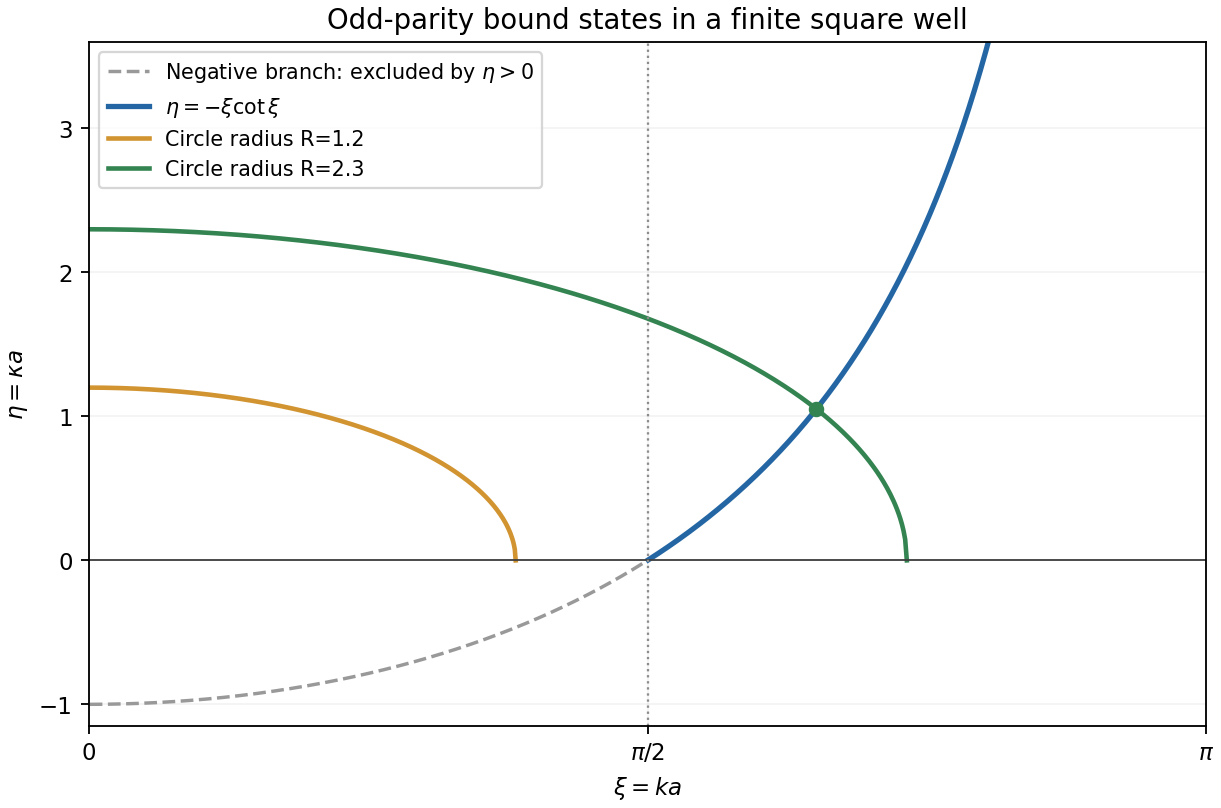
Past exam of the options II course of the University of Oxford 2010 G G2 Solution by Codex 0 2026-10-31
Codex 0 2026-10-31At a regular constrained extremal, the first variations satisfy for a constant Lagrange multiplier . One way to justify this is to choose a variation for which , use it to correct any other variation to preserve the constraint by the implicit function theorem, and differentiate along that corrected family. This gives the same ratio for all variations. The exceptional case for every variation requires the usual separate abnormal-extremal analysis.
Set . Integration by parts in its first variation givesTaking compactly supported variations and applying the fundamental lemma of the calculus of variations yields the Euler-Lagrange equation. For the quadratic integrands, it isor with . If endpoint values are free, independent endpoint variations give the natural conditionsAt a prescribed endpoint the variation instead vanishes and no natural condition is added there.
Under these natural conditions, integration by parts givesHence . For two solutions satisfying the same natural conditions, subtract their cross-multiplied equations and integrate:The final equality is the vanishing endpoint boundary form. Thus distinct eigenvalues giveThe same argument works for other common homogeneous boundary conditions making that boundary form zero.
In the Legendre case, . Comparing coefficients of in a degree- solution gives , so different degrees have different eigenvalues. A degree-zero solution is . A linear solution must be orthogonal to the nonzero constant solution, so and . Write . Orthogonality to gives , and orthogonality to gives . ThereforeThe constants are free normalization factors; for solutions of the stated exact degrees they are nonzero. The natural endpoint conditions hold automatically for these polynomials because .
Pinned article: Introduction to the OurBigBook Project
Welcome to the OurBigBook Project! Our goal is to create the perfect publishing platform for STEM subjects, and get university-level students to write the best free STEM tutorials ever.
Everyone is welcome to create an account and play with the site: ourbigbook.com/go/register. We belive that students themselves can write amazing tutorials, but teachers are welcome too. You can write about anything you want, it doesn't have to be STEM or even educational. Silly test content is very welcome and you won't be penalized in any way. Just keep it legal!
Intro to OurBigBook
. Source. We have two killer features:
- topics: topics group articles by different users with the same title, e.g. here is the topic for the "Fundamental Theorem of Calculus" ourbigbook.com/go/topic/fundamental-theorem-of-calculusArticles of different users are sorted by upvote within each article page. This feature is a bit like:
- a Wikipedia where each user can have their own version of each article
- a Q&A website like Stack Overflow, where multiple people can give their views on a given topic, and the best ones are sorted by upvote. Except you don't need to wait for someone to ask first, and any topic goes, no matter how narrow or broad
This feature makes it possible for readers to find better explanations of any topic created by other writers. And it allows writers to create an explanation in a place that readers might actually find it.
Figure 1. Screenshot of the "Derivative" topic page. View it live at: ourbigbook.com/go/topic/derivativeVideo 2. OurBigBook Web topics demo. Source. - local editing: you can store all your personal knowledge base content locally in a plaintext markup format that can be edited locally and published either:This way you can be sure that even if OurBigBook.com were to go down one day (which we have no plans to do as it is quite cheap to host!), your content will still be perfectly readable as a static site.
- to OurBigBook.com to get awesome multi-user features like topics and likes
- as HTML files to a static website, which you can host yourself for free on many external providers like GitHub Pages, and remain in full control

Figure 2. You can publish local OurBigBook lightweight markup files to either OurBigBook.com or as a static website.
Figure 3. Visual Studio Code extension installation.
Figure 5. . You can also edit articles on the Web editor without installing anything locally. Video 3. Edit locally and publish demo. Source. This shows editing OurBigBook Markup and publishing it using the Visual Studio Code extension. 
- Infinitely deep tables of contents:



All our software is open source and hosted at: github.com/ourbigbook/ourbigbook
Further documentation can be found at: docs.ourbigbook.com
Feel free to reach our to us for any help or suggestions: docs.ourbigbook.com/#contact