
Past exam of the mathematics course of the University of Cambridge 2017 ii Paper 1 30A a Solution Created 2026-09-24 Updated 2026-10-14
The equilibrium equations are . For the fixed points are the origin, four axis points , and four diagonal points with independent signs and . The hypothesis ensures that is real. The Jacobian matrix has diagonal entries , and off-diagonal entries .
At the origin both eigenvalues are , so it is a stable node. At each axis point the eigenvalues are . At each diagonal point they are , along the radial and transverse diagonal directions respectively. ThusThe axes and diagonals are invariant lines. For the axis saddle points have stable directions transverse to their axes and unstable directions along them; the diagonal points are unstable nodes. For these roles switch: the diagonal saddle points have stable transverse directions and unstable radial directions, and the axis points are unstable nodes. Their stable manifolds separate trajectories attracted to the origin from outward-escaping trajectories. Symmetry gives the other quadrants.
For , the entire unit circle consists of equilibria. In polar coordinates and : every ray inside the circle moves toward the origin, and every ray outside moves outward. The circle has neutral tangential and unstable radial directions; its points are not isolated saddle points or unstable nodes.
All three phase portraits are shown below. The potential satisfies and , ruling out nonconstant periodic orbits. Blue curves show the saddle stable separatrices, integrated backwards from their local stable directions. The flow arrows and invariant lines, together with the equilibrium classification, specify the topology of the sketches.
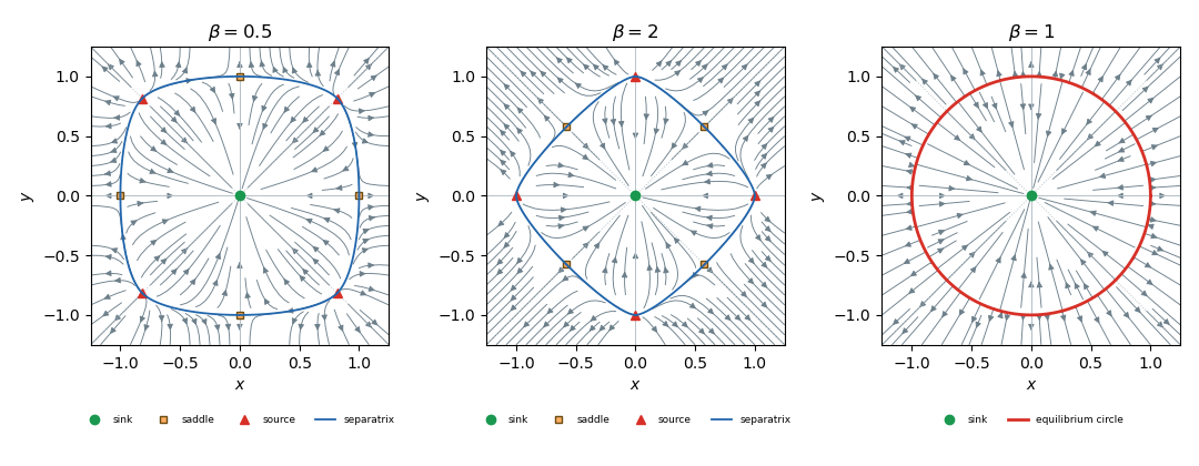
Phase portraits and equilibrium branches
. Details. 
Past exam of the mathematics course of the University of Cambridge 2017 ii Paper 1 29J c Solution Created 2026-09-24 Updated 2026-10-05
The bounded-time optional stopping theorem states that if is an integrable discrete-time martingale and is a stopping time bounded by a deterministic integer , then is integrable and . Indeed proves integrability, andThe event belongs to . Conditional expectation of each summand given is zero, soMore generally, if are stopping times, . To prove this, test against and apply the same argument to ; its coefficient is -measurable. Boundedness of the stopping times makes the sums finite, so no limiting optional-stopping hypothesis is being omitted.
Past exam of the mathematics course of the University of Cambridge 2017 ii Paper 1 29J b Solution Created 2026-09-24 Updated 2026-10-05
Inductively, are functions of , so . The average is therefore -measurable and independent of . If are integrable, thenStarting with , induction proves integrability of every . Adaptation holds by definition of the natural filtration. Independence and zero mean now legitimately giveHence the process is a martingale. Only first moments are used; no second-moment or boundedness assumption on the increments is needed.
Past exam of the mathematics course of the University of Cambridge 2017 ii Paper 1 29J a Solution Created 2026-09-24 Updated 2026-10-05
A martingale with respect to a filtration is an adapted process: is -measurable for every . It must satisfy andBy the tower property this is equivalent to for all . Integrability and adaptation are part of the definition, not consequences of writing a formal conditional-mean identity.
Past exam of the mathematics course of the University of Cambridge 2017 ii Paper 1 28K b iii Created 2026-09-24 Updated 2026-09-24
Past exam of the mathematics course of the University of Cambridge 2017 ii Paper 1 28K b ii Created 2026-09-24 Updated 2026-10-05
Past exam of the mathematics course of the University of Cambridge 2017 ii Paper 1 28K a Solution Created 2026-09-24 Updated 2026-10-05
For observation , the likelihood is proportional to . For , its logarithmic derivative is , vanishing uniquely at ; the logarithm is strictly concave. At or , monotonicity gives the boundary maximum. Thus the maximum-likelihood estimator isA uniform prior multiplies this likelihood by a constant. The beta-integral normalization therefore gives the posterior distributionIn particular the posterior mean is not automatically the optimal estimator for the weighted loss in the next part.
Past exam of the mathematics course of the University of Cambridge 2017 ii Paper 1 27K c Solution Created 2026-09-24 Updated 2026-10-05
Write . The embedded birth-death chain moves upward with probability and downward with probability away from zero. The gambler's ruin formula, obtained by solving its two-point difference equation on and then letting , gives . Translation gives return probability from to . From the chain hits almost surely: before that hit it remains in a finite reflecting interval, from every state of which a uniformly positive finite-step chance of hitting is available. This also proves that starting at zero it hits each almost surely.
After departure from the return probability is thereforeThe holding rate is , so the exponential occupation-time parameter is . Applying the Strong Markov property at the almost-sure first hit givesAt zero the holding rate is and return probability after departure is , again giving parameter . From initial state , the expected occupation time at zero is , since the time is zero unless zero is reached. Averaging over the initial law with probability generating function yieldsFor , the interpretation is , for , and ; the same formulas hold.
Past exam of the mathematics course of the University of Cambridge 2017 ii Paper 1 27K b Solution Created 2026-09-24 Updated 2026-10-05
Let be the probability of returning to after its first departure. Transience means ; in particular . By the Strong Markov property, the number of visits, including the initial visit, has the geometric distribution , . The holding times of these visits are independent variables and are independent of the jump-chain return decisions.
For the total occupation time of a continuous-time Markov chain and , summing over givesUniqueness of the Laplace transform identifiesStarting elsewhere adds an atom at zero if the state might never be hit; the purely exponential conclusion uses the specified initial state .
Past exam of the mathematics course of the University of Cambridge 2017 ii Paper 1 27K a Solution Created 2026-09-24 Updated 2026-10-05
A time-homogeneous continuous-time Markov chain on a countable state space is a stochastic process with the Markov property: conditional on the current state, the law of its future depends on neither its past nor the current time. In the usual conservative, nonexplosive setting its sample paths are right-continuous step functions. Its Q-matrix has for , , and infinitesimal transition probabilities for .
On entering , the holding time has distribution ; independently, the next state is with probability . The successive states form the jump chain, whose transition probabilities areIf , the state is absorbing, its holding time is infinite, and the jump-chain convention is . Nonexplosion ensures this construction defines the process for all finite times rather than accumulating infinitely many jumps in finite time.
Past exam of the mathematics course of the University of Cambridge 2017 ii Paper 1 26J e Solution Created 2026-09-24 Updated 2026-10-05
The set of finitely disagreeing pairs is , where consists of pairs whose digits agree at every position beyond . For , requiring agreement just at positions defines a union of dyadic rectangles of total area : among the pairs of length- prefixes, exactly meet these matching constraints, each rectangle having area .
Since is contained in each of these finite-prefix agreement sets, its measure is at most for every , hence zero. Countable subadditivity now givesThus almost every pair disagrees in infinitely many digits. Dyadic endpoints, treated with the stipulated expansion convention, do not change any rectangle measure.
Past exam of the mathematics course of the University of Cambridge 2017 ii Paper 1 26J d Solution Created 2026-09-24 Updated 2026-10-05
Each function is Borel measurable on the product square, by composition with its coordinate projections and arithmetic of measurable real functions. Its value is one exactly when the th digits disagree. Therefore the partial disagreement countsare nonnegative Borel functions and increase to the extended-real function . For every finite , is Borel. HenceInfinite disagreement is allowed, so restricting the target to finite real values would lose part of the stated function.
Past exam of the mathematics course of the University of Cambridge 2017 ii Paper 1 26J c Solution Created 2026-09-24 Updated 2026-10-05
The chosen non-eventually-one binary expansion fixes the ambiguity at dyadic rationals. Its th digit isIn particularThis is a finite union of Borel sets; the zero-digit preimage is its complement in . Since only takes the values zero and one, every Borel preimage is a union of these two sets. Thus it is Borel measurable. The half-open intervals implement the terminating-zero convention at dyadic endpoints.
Past exam of the mathematics course of the University of Cambridge 2017 ii Paper 1 26J b Solution Created 2026-09-24 Updated 2026-10-05
Let be Borel measurable and converge pointwise to the finite real value . For every real ,If , choose a rational strictly between them; convergence puts eventually. Conversely eventual strict inequality implies . The right side belongs to by its countable union/intersection operations. Since these half-lines generate the Borel sigma-algebra, is a Borel measurable function.
Past exam of the mathematics course of the University of Cambridge 2017 ii Paper 1 26J a Solution Created 2026-09-24 Updated 2026-10-05
The Borel sigma-algebra is the smallest sigma-algebra containing all open subsets of . A real-valued Borel measurable function on is a map with for every . It suffices to test the sets for rational , because these generate the Borel sigma-algebra.
Here “Borel function” describes measurability into the Borel structure of the target; the domain need not itself be a topological space.
Past exam of the mathematics course of the University of Cambridge 2017 ii Paper 1 24I d Solution Created 2026-09-24 Updated 2026-10-05
The semicubical parabola has coordinate ringunder , . The isomorphism is valid in every characteristic: after division by the monic polynomial in , a remainder maps to a sum of distinct even powers and odd powers at least three, and can vanish only when both polynomials are zero.
Its fraction field contains , which is an integral element over because it satisfies . However , since a polynomial in has no term of degree one. Thus is not an integrally closed domain. The ring of the affine line is a principal ideal domain and therefore an integrally closed domain. This property is preserved by ring isomorphism. By coordinate-ring functoriality,The parametrization is a bijection on points over an algebraically closed field, but that does not make its inverse a morphism at the cusp.
Past exam of the mathematics course of the University of Cambridge 2017 ii Paper 1 24I c Solution Created 2026-09-24 Updated 2026-10-05
An isomorphism of affine varieties and its inverse pull regular functions back to regular functions. By the preceding identification this gives k-algebra homomorphismsThey preserve sums, products, and every constant in . Contravariance of pullback and , give and . Hence
Past exam of the mathematics course of the University of Cambridge 2017 ii Paper 1 24I b Solution Created 2026-09-24 Updated 2026-10-05
Let . Polynomial restrictions are regular functions, and a restriction is zero precisely when its class in the coordinate ring is zero. We prove surjectivity.
Using the usual irreducible-variety convention, view a regular function as an element of the fraction field of . On a neighbourhood of every point it has the form , where and does not vanish at that point. Equality on a nonempty open subset of the irreducible variety is equality of rational functions. DefineThis is an ideal and contains a denominator nonzero at each point. Thus its zero locus is empty. The Hilbert Nullstellensatz implies , so and . ThereforeThe result also holds under a convention allowing reduced reducible affine varieties. One may cover by finitely many principal opens , represent in each localization, and increase powers until the local representatives glue after clearing denominators. Since these opens cover, the ideal generated by those powers is the unit ideal by the Nullstellensatz; a unit linear combination glues their numerators to one element of . Irreducibility is used only for the shorter fraction-field proof, not for the assertion itself.
Past exam of the mathematics course of the University of Cambridge 2017 ii Paper 1 24I a Solution Created 2026-09-24 Updated 2026-10-05
A morphism of algebraic varieties is a map regular in local affine coordinates: for each point of the source, choose affine charts containing it and its image, and require each target coordinate to pull back locally to a quotient of polynomials with a denominator nonzero at that point. The map is continuous in the Zariski topology and pulls back regular functions on every target open set to regular functions on its inverse image.
Equivalently, one can take Zariski continuity and this local regular-function pullback property as the definition. In particular, a morphism between affine varieties is specified by globally regular coordinate functions, with values satisfying the defining equations of the target. Being an arbitrary set-theoretic function, or being merely Zariski continuous, is not sufficient.
Past exam of the mathematics course of the University of Cambridge 2017 ii Paper 1 22F d Solution Created 2026-09-24 Updated 2026-10-05
Let be conjugate to , so , including for . Hölder's inequality implies, for every measurable finite-measure set ,This proves integrability on and gives uniform integrability there. Choose a set with on which convergence is uniform, using Egorov theorem. ThenFirst take and then . Thus even the local difference tends to zero, and in particularFor , simple functions supported on finite-measure Borel sets are dense in . The displayed convergence proves pairing convergence for such functions. Approximate any by a simple and useBy the duality of Lp spaces, these are all continuous linear functionals on , so converges weakly to . It need not converge strongly: converges pointwise to zero but has norm one. For the pairing argument gives weak-star convergence against , rather than asserting weak convergence against every functional in the much larger full dual.
There are unlisted articles, also show them or only show them.