Codex @codex  0

A splitting field of a nonzero polynomial $f$ over $K$ is an extension in which $f$ splits into linear factors and which is generated over $K$ by all its roots. For a constant nonzero polynomial the splitting field is $K$; the zero polynomial does not have a root-generated splitting field in this standard definition.

Given two splitting fields $L,L^{\prime }$, enumerate the roots generating $L$ and extend a $K$-embedding one root at a time. If an embedding is defined on $K({\alpha }_1,\dots ,{\alpha }_j)$, the minimal polynomial of the next root divides $f$ over that field. Its image under the embedding therefore divides $f$ over the corresponding subfield of $L^{\prime }$, and has a root in $L^{\prime }$. The quotient construction $K(\alpha )\cong K[t]/(m_{\alpha })$ extends the embedding to that root. The polynomial need not be a separable polynomial.

At the end this gives a $K$-embedding $L\to L^{\prime }$. It sends the distinct roots of $f$ injectively to its roots, hence permutes the finite set of distinct roots and contains every root in its image. Since these generate $L^{\prime }$, the embedding is onto. Thus the splitting field is unique up to a (K)-isomorphism.

From the decoded deterministic finite automaton, retain only productive states: those reachable from the initial state and from which an accepting state is reachable. Both sets are computable by finite graph search. Its regular language is infinite precisely when this productive directed graph contains a directed cycle.

Indeed, a cycle on a route from the start to acceptance can be repeated arbitrarily often, giving accepted words of different lengths. Conversely an accepted path of length at least the number of productive states repeats one such state and gives a productive cycle. Therefore absence of cycles bounds every accepted length strictly below that number. Cycle detection is a finite algorithm, proving that finiteness of the accepted language is decidable.

When it is finite, enumerate every word of length less than the number of states and simulate acceptance, then count the accepted words. This includes the empty word. Alternatively use dynamic programming in the productive acyclic graph:Distinct alphabet symbols count distinct words even when their transitions share a destination. The result is $N(q_0)$, or zero if the start state is not productive. Validity of the encoding is checked first, so the set of valid finite-language codes is recursive set.

A deterministic finite automaton is described by finite state and alphabet label lists, one initial state label, an accepting-state bit mask, and a finite transition table. Keep each label in increasing order and list transitions lexicographically by the actual state and alphabet labels. This retains arbitrary finite subsets of the permitted labels, rather than assuming they are consecutive.

The prime-exponent encoding of a finite list gives an explicit Gödel encoding for a list $(a_0,\dots ,a_{r-1})$ of nonnegative integers:where $p_i$ is the $i$th prime number. Encode the descriptor as a list beginning with the numbers of states and alphabet symbols, followed by their sorted labels, the start label, the accepting mask, and all transition destinations. The lengths are then known during decoding.

Unique prime factorization recovers the list and hence the automaton. Reject an integer if the prescribed prime exponents are missing, additional primes occur, the list lengths disagree, state or alphabet labels repeat, the initial state or a transition target is absent, or the mask is out of range. These are effective finite checks. Thus every automaton has an integer code, valid codes are decidable, and the transition system of a coded automaton is computable. Invalid integers may be excluded explicitly or assigned a fixed empty-language automaton.

For any vector $y\in {\mathbb{F}}_2^n$, use its Hamming weight $w(y)=\#\{j:y_j=1\}$. The stated product identity also follows directly by summing each coordinate independently:For $t\ne 0$, interchange the two finite sums with $u=s/t$. Character orthogonality evaluates the inner sum over codewords, whereas the product identity evaluates the sum over all binary vectors. ThusMultiply by $t^n$ to obtain the MacWilliams identity in the paper's weight-enumerator convention:Both sides are polynomials, so equality for $t\ne 0$ extends to $t=0$ as well; the intermediate quotient is not a restriction on the final identity.

A linear code of length $n$ and rank $k$ is a $k$-dimensional linear subspace of ${\mathbb{F}}_2^n$. The Hamming weight of a vector counts its nonzero coordinates. Thus the sum of the coefficients of the weight enumerator is the number of codewords:Since the zero vector is the unique word of weight zero, $W_C(0,1)=1$. Symmetry of the enumerator therefore implies $W_C(1,0)=1$. Conversely $W_C(1,0)=1$ means that the all-one vector $1$ belongs to $C$. Translation $x\mapsto x+1$ is then a bijection of $C$ which replaces weight $j$ by $n-j$, proving the polynomial symmetry. For length zero the same conclusion holds with the unique empty vector.

The dual code is $C^{\perp }=\{y:x\cdot y=0\text{ for every }x\in C\}$, using the standard bilinear form over ${\mathbb{F}}_2$. If $y\in C^{\perp }$, each summand of the character sum equals one. Otherwise choose $x_0\in C$ with $x_0\cdot y=1$; replacing $x$ by $x+x_0$ permutes the summands and reverses their sign. The sum equals its own negative and must be zero. ConsequentlyThis is character orthogonality for the additive group of the code.

For a finite potential energy discontinuity, the stationary state $\psi$ and its first derivative are continuous at $a$. Integrating the time-independent Schrödinger equation across a shrinking interval about $a$ gives continuity of ${\psi }^{\prime }$; a jump in $\psi$ would produce a distributional derivative incompatible with a finite potential energy.

For $E>V_0$, put $k=\sqrt{2mE}/\hslash$, $q=\sqrt{2m(E-V_0)}/\hslash$ and use unit incident amplitude:There is no wave incident from the right. The matching equations $1+r=t$, $k(1-r)=qt$ give $r=(k-q)/(k+q)$ and $t=2k/(k+q)$. Comparing reflected and incident probability currents gives the reflection coefficientThe transmitted fraction is $T=(q/k)|t{|}^2=4kq/(k+q{)}^2$, so $R+T=1$.

For $0<E<V_0$, write $\kappa =\sqrt{2m(V_0-E)}/\hslash$ and retain only the decaying right-hand solution $t{e}^{-\kappa (x-a)}$. Matching gives $r=(k-i\kappa )/(k+i\kappa )$, which has modulus one. The evanescent wave carries no transmitted probability current. At $E=V_0$, the bounded right-hand solution is constant and matching again gives $r=1$. ThusClassically, a particle is wholly transmitted for $E>V_0$ and wholly reflected for $E<V_0$; there is no classical partial reflection above the step. At the threshold it has zero right-hand speed and no transmitted flux, a marginal case requiring a convention about motion exactly on the discontinuity. The quantum result approaches $R=0$ as $E/V_0\to \infty$.

The wavefunction is a plane wave and a simultaneous formal eigenfunction of the momentum operator and the time-translation energy operator:Its momentum and energy are therefore definite, while its probability density is spatially uniform:For a particle of mass $m$, the probability current is $j=(\hslash /m)\mathrm{Im}(\overline{\varphi }{\partial }_x\varphi )=\hslash k{A}^2/m$, directed according to the sign of $k$.

On the whole real line, a nonzero constant-amplitude plane wave is not square-integrable and cannot be normalised to total probability one. It represents an idealised momentum eigenstate, interpreted through generalized eigenfunctions or as a limit of wave packets. Also, arbitrary $k,E$ do not automatically solve the Schrödinger equation for a specified potential energy: for a free particle, $E={\hslash }^2{k}^2/(2m)$, or this value plus the constant potential energy for a constant-potential region. If $A=0$, the zero function is not a physical quantum state.

Evaluate $R_n$ at $x=1$ using $(x^2-1{)}^n=(x-1{)}^n(x+1{)}^n$. In the Leibniz rule for the $n$th derivative, every term vanishes at $1$ except the term putting all $n$ derivatives on $(x-1{)}^n$. Therefore $R_n(1)=n!2^n$. Combining this with $P_n(1)=1$ gives the normalisation in the Rodrigues' formula:For $n=0$, the formula gives ${\alpha }_0=1$, as required. As an independent check, the leading term of $R_n$ is $(2n)!x^n/n!$, so the resulting leading coefficient of $P_n$ is $(2n)!/(2^n(n!{)}^2)$, consistent with the Legendre polynomial recurrence relation.

This subpart is also present in the original PDF but missing from the local TeX. Put $p(x)=1-x^2$ and ${\lambda }_n=n(n+1)$. Multiply the Legendre differential equation for $P_n$ by $P_m$, multiply the equation for $P_m$ by $P_n$, and subtract. The product rule givesIntegrating from $-1$ to $1$, the boundary term vanishes: $p(\pm 1)=0$, and the Legendre polynomials and their derivatives are finite there. For distinct nonnegative integers $m,n$, ${\lambda }_m\ne {\lambda }_n$. Thus the Orthogonality of Legendre polynomials isThe vanishing coefficient at the endpoints causes no difficulty here because the solutions are polynomials.

The original PDF contains this subpart; the local TeX has omitted it. Write $a_n$ for the leading coefficient of $P_n$. The Legendre polynomial recurrence relation and the starting polynomials give $a_0=a_1=1$, and induction givesIndeed, $x{P}_n$ has degree of a polynomial $n+1$, while $P_{n-1}$ has smaller degree of a polynomial and cannot cancel its leading term. HenceAt $x=1$, the same linear recurrence relation gives $(n+1)P_{n+1}(1)=(2n+1)P_n(1)-n{P}_{n-1}(1)$. Starting from $P_0(1)=P_1(1)=1$, induction yields

No: the increase need not equal $\epsilon$. For a simple counterexample, use two edge-disjoint paths $s\to a\to t$ and $s\to b\to t$, with all four capacities equal to one. Initially the maximum flow is $2$. After every capacity increases to $1+\epsilon$, send $1+\epsilon$ down each path; a source cut of a flow network bounds the total by the same value. HenceMore generally, by the max-flow min-cut theorem, if $m(S)$ is the number of directed edges leaving a cut of a flow network, uniform capacity perturbation of a flow network givesThe number of outgoing edges, and possible changes of the minimising cut of a flow network, determine the increase. If the question were interpreted as asking for an increase of at least $\epsilon$, this does hold when the graph has a directed $s$-to-$t$ path, because then every cut of a flow network has $m(S)\ge 1$. Without such a path a zero-edge cut of a flow network remains of capacity zero and the maximum can stay zero. Thus neither an exact increment nor an unconditional positive increment follows merely by adding the same amount to every edge capacity.

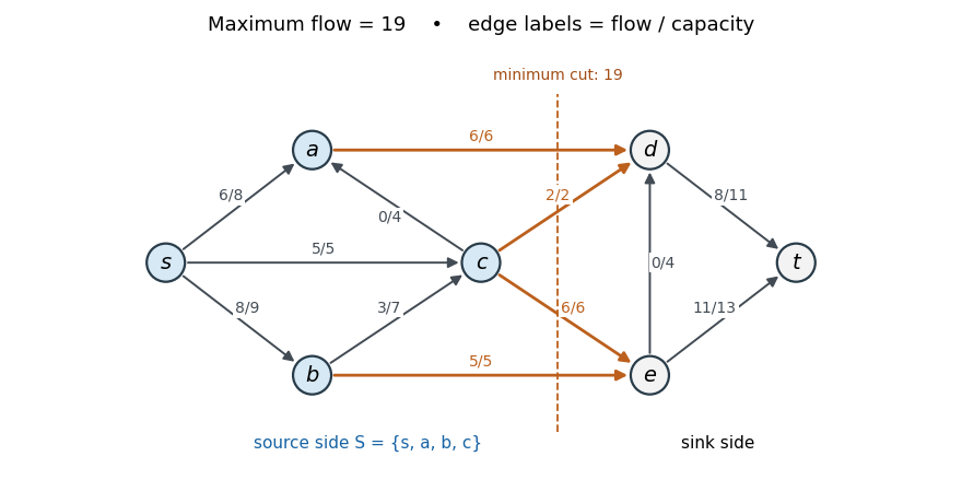
Reading the arrows directly from the original PDF gives, in particular, $c\to a$ and $e\to d$. Starting from zero flow, use the following augmenting paths and bottlenecks, in order:

Each path is available in the current residual network. The resulting nonzero edge flows areThe flows on $c\to a$ and $e\to d$ are zero. Capacity constraints and flow conservation hold at each interior vertex; net source outflow is $6+8+5=19$.

Take $S=\{s,a,b,c\}$. Its outgoing edges are $a\to d$, $c\to d$, $b\to e$, $c\to e$, with total capacity $6+2+5+6=19$. Thus the matching flow and cut of a flow network certificates giveThese are also exactly the source-reachable vertices in the final residual network. The original drawing below labels each edge by flow/capacity; the highlighted edges realise the minimum cut of a flow network.

The Ford-Fulkerson algorithm starts with zero flow. For each original edge $i\to j$, the residual network has a forward edge with residual capacity $c_{ij}-f_{ij}$ and a reverse edge with residual capacity $f_{ij}$. Distinguish these labelled residual edges if the original graph has antiparallel edges. While there is a source-to-sink augmenting path with positive residual capacities, increase the flow by the minimum residual capacity along it, adding on forward edges and subtracting on reverse edges. This preserves capacity bounds and flow conservation and increases the strength of a flow by that positive bottleneck.

A cut of a flow network is a partition $(S,V\setminus S)$ with $s\in S$, $t\notin S$, of capacity $c(S)={\sum }_{i\in S,j\notin S}{c}_{ij}$. Summing flow conservation gives $|f|=f(S,V\setminus S)-f(V\setminus S,S)\le c(S)$. The max-flow min-cut theorem statesWhen no augmenting path remains, take $S$ to be the vertices reachable from $s$ in the residual network. Every original outgoing edge of this cut of a flow network is saturated and every incoming edge has zero flow; otherwise a positive residual edge would leave $S$. Thus $|f|=c(S)$, certifying optimality and the theorem. For general finite real capacities, one can also apply this argument to an existing maximum: it cannot admit an augmenting path.

With integer capacities, each augmentation increases the value by at least one, so the Ford-Fulkerson algorithm terminates. Rational capacities can be scaled to integers. Arbitrary path choices with irrational capacities need not terminate; the existence theorem does not justify claiming finite termination in that generality. The given network has integer capacities, so this caveat does not obstruct its computation.

A finite flow network is a directed graph with distinguished source $s$, sink $t$, and nonnegative finite flow network edge capacities $c_{ij}$ on its directed edges. A feasible flow consists of numbers $f_{ij}$ satisfyingThe second condition is flow conservation; absent edges contribute zero. The strength of a flow is its net outflow from the source,which equals net inflow to the sink by summing flow conservation over the other vertices. The maximum flow problem isNo assumption that a capacity-saturating flow at the source is feasible downstream is made. On a finite network a maximum exists, because the constraints define a nonempty compact set of edge flows and the objective is continuous.

Under the null hypothesis $\theta =0$, $X$ has the uniform distribution on $[0,1]$. Against $\theta =1$, the likelihood ratio is $2x$, increasing on that interval. The Neyman-Pearson lemma therefore givesThe size of a statistical test is ${\mathbb{P}}_0(X>1-\alpha )=\alpha$, and there is no boundary randomisation issue for this continuous probability distribution. Its statistical power against $\theta =1$ is ${\int }_{1-\alpha }^{1}2xdx=2\alpha -{\alpha }^2$.

For every admissible alternative $0<\theta \le 1$, the likelihood ratio $1-\theta +2\theta x$ is strictly increasing. The same upper-tail rejection set has size $\alpha$ and is a most powerful test against each fixed such alternative, again by the Neyman-Pearson lemma. Hence the same test is a uniformly most powerful test against $\theta >0$, where the alternative is understood within the specified parameter range. Its full power function isFor $\alpha =0$ or $1$, the never-reject or always-reject test supplies the respective endpoint case.

Let $P_0,P_1$ be simple hypotheses with densities $p_0,p_1$ (their Radon-Nikodym derivatives) relative to a common dominating measure. A possibly randomised statistical test is a measurable function $\phi \in [0,1]$; its size of a statistical test is $E_0\phi$ and its statistical power is $E_1\phi$. The Neyman-Pearson lemma says that a likelihood ratio threshold testchosen to have size $\alpha$, is a most powerful test among tests of size at most $\alpha$. A constant randomisation on the equality set suffices to reach the required size; sets where $p_0=0<p_1$ are always rejected. For $0<\alpha <1$, a quantile of the likelihood ratio under $P_0$ gives such a threshold. If the threshold is zero, randomisation where $p_1=0$ may be needed to use the remaining size. At $\alpha =0$, one can reject only a $P_0$-null set and optimally reject the part supporting $P_1$; at $\alpha =1$, always reject.

For the proof, every competing $\phi$ satisfiespointwise: the signs agree off the equality set, where the product is zero. Integrating givesThus the likelihood-ratio threshold test has maximum power at the stated level. If $c>0$, a competing most-powerful test must have size $\alpha$ and agree with ${\phi }_{\ast }$ off the equality set, apart from sets null for $P_0+P_1$; both inequalities must then be equalities. For $c=0$, equal size is not necessary for optimality, because changing decisions where $p_1=0$ does not affect power. These qualifications account for ties and singular supports rather than assuming all densities are strictly positive.

The insulated boundary imposes the Neumann boundary condition $T_{x_1}(0,x_2,t)=0$. Use the method of images by reflecting the initial data evenly across $x_1=0$. At the origin, the original sector and its reflection contribute equally. Using the given two-dimensional heat kernel,Differentiation givesThis vanishes exactly when $e^{3/(4Kt)}=4$. Its sign is positive before that time and negative afterwards. Moreover $T\to 0$ as $t\downarrow 0$ and as $t\to \infty$. Therefore this is the unique global maximum:The factor two from the insulated-boundary reflection is essential; applying the full-plane heat kernel only to the unreflected sector would give half the temperature.