
Past exam of the mathematics course of the University of Cambridge 2010 ii Paper 2 8E Solution Created 2026-09-24 Updated 2026-10-14
The removable singularities at zero are understood inThese are entire functions, with values and . On the real axis their difference is , including its continuous value at zero. In the complex upper half-plane, , so away from zero; the analogous bound for holds in the lower half-plane. This verifies analyticity, the required jump and the specified decay.
In the Sokhotski–Plemelj formula, the boundary values may also be writtenIndeed the Cauchy principal value of is : split , translate the first integral, and use and the oddness of . The limiting formula at zero follows continuously.
Past exam of the mathematics course of the University of Cambridge 2010 ii Paper 2 7D Solution Created 2026-09-24 Updated 2026-10-14
The only equilibrium point is . Its Jacobian matrix is , with characteristic polynomial . For both eigenvalues have negative real parts, so the origin is locally asymptotically stable.
Use the Lyapunov function . Along a solution,A Lyapunov function is positive away from the equilibrium and nonincreasing along trajectories; its sufficiently small sublevel sets prove stability. Asymptotic stability additionally means nearby trajectories converge to the equilibrium. The basin of attraction is the set of initial states whose forward solutions exist for all positive time and converge to it. Every closed disc of radius at most is positively invariant, since there. The LaSalle invariance principle says that a solution in a compact positively invariant set where approaches the largest invariant subset of . Here that subset is only the origin: on , remaining on the line would require ; the isolated points on the outer disc do not remain there because . Hence the closed disc lies in the basin of attraction.
This estimate does not assert that the basin is exactly that disc, or the whole plane. For example, choose so large that and . The region is positively invariant: on one has , and on one has . Within it , which forces finite-time escape. Thus the attraction is genuinely local. The Lyapunov function gives a rigorous sufficient domain for attraction without identifying its entire boundary.
Past exam of the mathematics course of the University of Cambridge 2010 ii Paper 2 6A Solution Created 2026-09-24 Updated 2026-10-14
Write , with . Besides zero, the fixed points satisfy . If , they areThe derivative is . At a positive fixed point, , so . Thus zero is attracting, is repelling because , and is attracting because .
Moreover,For the iterates strictly decrease and stay positive. Their limit is a fixed point below , hence zero. For the iterates increase towards ; for they decrease towards . Monotonicity of prevents crossing the limiting fixed point. is the extinction threshold. The cobweb plot illustrates these alternatives.
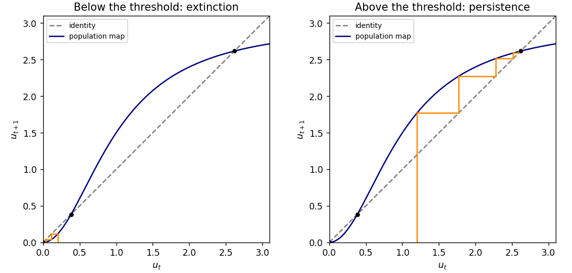
Population cobwebs below and above the unstable extinction threshold
. Details. 
For there are no positive fixed points, and for every , so all populations tend to zero. At , the positive fixed point is semistable: initial populations below it tend to zero, and those above it decrease towards it. This is a saddle-node bifurcation in the discrete dynamics.
Past exam of the mathematics course of the University of Cambridge 2010 ii Paper 2 5J Solution Created 2026-09-24 Updated 2026-10-14
A maximum-likelihood estimator maximizes the likelihood as a function of the parameter for the observed data. Under the usual regularity conditions, a scalar maximum-likelihood estimator satisfies , where is the Fisher information in one observation.
For a Poisson distribution with , the log-likelihood is . Solving gives . Its expectation is and its variance is . If all observations are zero, the maximum over occurs at zero; over this is a boundary supremum. The one-observation score function is , so and the asymptotic variance of is .
For , let . The identitygives , so is another unbiased estimator. However, the total score function has variance . For any regular unbiased estimator , differentiating gives , so the Cauchy-Schwarz inequality yields . The sample mean attains this Cramér-Rao bound exactly. There is no variance advantage in preferring to .
Past exam of the mathematics course of the University of Cambridge 2010 ii Paper 2 4H Solution Created 2026-09-24 Updated 2026-10-14
Take the parity-check matrixover . Its columns are all the nonzero vectors of . The Hamming code is . Since has rank three, is a binary linear code of length seven and dimension four. No nonzero codeword has weight one or two, since no column is zero and no two columns coincide. Columns give a codeword of weight three, so has parameters .
For a received vector , its syndrome is . A single error in position gives exactly column of , so the syndrome identifies that position uniquely; zero syndrome means no error under the one-error assumption. The radius-one Hamming balls around the codewords are disjoint and have total size , so this is also a perfect code.
There are weight-three codewords: every pair of columns determines the third, and each triple is counted three times. The all-ones vector is a codeword because the column sum is zero, so complementation gives seven weight-four codewords. Together with zero and the all-ones vector these account for all sixteen. The weight enumerator is therefore
Past exam of the mathematics course of the University of Cambridge 2010 ii Paper 2 3F Solution Created 2026-09-24 Updated 2026-10-14
Let and . The Euclidean isometry fixes the origin and preserves norms. The polarization identity therefore gives . In particular, are an orthonormal basis. The coefficients of in this basis are , so . Thus is a linear map represented by an orthogonal matrix, and . Conversely, every such map preserves distances because .
When , the real eigenvalues of the two-dimensional orthogonal matrix are . Choose corresponding unit eigenvectors , and write . In these coordinates . This is reflection in the line , followed by translation along that line. It is a Euclidean reflection if , and a glide reflection if .
Past exam of the mathematics course of the University of Cambridge 2010 ii Paper 2 39A Solution Created 2026-09-24 Updated 2026-10-14
Use the printed unnormalized inverse discrete Fourier transform, with positive exponent: . Its natural domain and codomain are ; the printed real-to-real designation is not literal, as the first example below has complex output. There is no factor in the convention of this question.
Past exam of the mathematics course of the University of Cambridge 2010 ii Paper 2 38A Solution Created 2026-09-24 Updated 2026-10-14
Taking the divergence and curl of the elastic equation givesSubstitution of the plane wave gives . Resolve parallel and perpendicular to . A P wave has longitudinal polarization and ; an S wave has transverse polarization and , with two transverse polarizations.
For the Rayleigh wave, take displacement potentials in the plane,where , . For , both waves decay into . These are an evanescent longitudinal wave and an evanescent vertically polarized shear wave. At , the Cauchy stress tensor givesThe third traction component is already zero. The two remaining stress-free conditions have a nonzero solution exactly when their determinant vanishes:Substituting gives the required Rayleigh wave equation. The nonzero subsonic root supplies a self-sustained surface wave; no existence proof for that root is required. The formal zero-speed root is degenerate and does not describe a propagating wave.
Past exam of the mathematics course of the University of Cambridge 2010 ii Paper 2 37A Solution Created 2026-09-24 Updated 2026-10-14
The lubrication approximation applies in a gap thin compared with its horizontal scale, with small slopes, no slip at the walls, negligible inertia, and approximately constant pressure across the gap. Continuity makes the horizontal velocity much larger than the normal velocity. At , write , where and keeps the gap open.
The horizontal Stokes equation becomes . Both plates have zero horizontal velocity, soIntegrated incompressibility with the moving upper wall gives . Since , , and , giving .
Past exam of the mathematics course of the University of Cambridge 2010 ii Paper 2 36B Solution Created 2026-09-24 Updated 2026-10-14
Use metric compatibility and the symmetric Levi-Civita connection. Expanding givesThe Christoffel formula makes the bracket . Thus the Killing equation is equivalent to the displayed coordinate formula in the question, also the vanishing Lie derivative of the metric.
Along an affinely parametrized geodesic with tangent ,The first term vanishes by the geodesic equation and the second by the Killing equation, because is symmetric. This proves the geodesic conserved quantity from a Killing vector.
For , the three independent coordinate Killing conditions areThe field satisfies all three immediately. For , the second equation reads , and the third reads . For , they read and . The first equation holds for both, verifying all three Killing vector fields.
Their conserved contractions with may be denotedAdding the last two expressions after multiplying by givesTo identify these loci, set , . The metric becomes , and the equation becomes , a straight line in Minkowski spacetime. Nontrivial such lines, parametrized affinely, are exactly the geodesics in this coordinate patch. The all-zero choice of constants is a vacuous equation rather than an individual geodesic.
Past exam of the mathematics course of the University of Cambridge 2010 ii Paper 2 35C Solution Created 2026-09-24 Updated 2026-10-14
Each one-particle momentum state occupies volume in momentum space. Counting the spherical shell gives the density of statesThe increasing dispersion law permits inversion, and the density is zero below any minimum allowed energy. No additional spin degeneracy is included here.
For noninteracting particles, the classical Boltzmann sum factorizes into . Dividing by accounts for indistinguishability without quantum exchange corrections, giving the partition function , with . Differentiation with respect to inverse temperature givesFixed mode indices have momenta proportional to because the boundary quantization condition fixes . As , and . The pressure , evaluated by differentiating the mode sum, therefore obeys
The nonrelativistic thermal wavelength is , and . If , then : occupation per thermal quantum state is small. Wave packets scarcely overlap and exchange corrections to Maxwell-Boltzmann distribution are negligible, justifying the classical formulas.
Past exam of the mathematics course of the University of Cambridge 2010 ii Paper 2 34B Solution Created 2026-09-24 Updated 2026-10-14
The asymptotic scattering wavefunction is . For a real central potential, the scattering phase shift multiplies the outgoing component of each partial wave relative to the incoming one by . Matching the incident-wave normalization givesSubtract the given incident plane wave expansion. Since , the scattering amplitude isOrthogonality eliminates cross terms in , giving .
For the spherical square well, the regular reduced radial wave is inside and outside, with . Continuity of the wave and its derivative gives the logarithmic-derivative matching relation , orAt zeros of the denominators the original matching relation supplies the limiting interpretation.
Under the stated deep-well approximation, put and . The condition is . If , its first positive solution lies in ; if , it is . For , a solution lies in because there rises continuously from zero to infinity. If , the first positive solution lies in , where rises from one to infinity. The limiting pole case gives by the cotangent relation. Thus , without calculating the integer phase index. The use of presumes the located wave numbers remain small compared with .
Past exam of the mathematics course of the University of Cambridge 2010 ii Paper 2 33C Solution Created 2026-09-24 Updated 2026-10-14
The rotation unitary operator is . A state with zero orbital angular momentum has a rotationally invariant orbital factor; a spinless state is wholly unchanged. Zero orbital angular momentum alone does not rule out a nontrivial rotation of intrinsic spin angular momentum.
For spin one-half, . Direct multiplication of the Pauli matrices gives . The antisymmetric part vanishes when contracted with , henceFor , the operator has trace zero, so its eigenvalues are ; for both are zero. With unit , the even and odd powers in the exponential give
Take . The rotated state satisfies , because . By the Born rule, the probability of this outcome in the initial state is . In the eigenbasis,The transition from to thus has probability . .
Past exam of the mathematics course of the University of Cambridge 2010 ii Paper 2 32E Solution Created 2026-09-24 Updated 2026-10-14
Insert the finite exponential expansion into the Gelfand-Levitan-Marchenko equation. The integral contribution isComparing coefficients of givesFor this coefficient comparison take the distinct; repeated exponents can first be combined. The linear system supplies the coefficients whenever its matrix is invertible.
In the inverse scattering transform convention , the Korteweg-De Vries equation solution is . The reflectionless scattering data evolve as , with the fixed. For one exponential,Differentiating its diagonal givesFor , this is the smooth solitonIt travels at speed . If the solution is zero; if the denominator vanishes somewhere, so the formula is not a globally smooth one-soliton. Positivity is the necessary qualification for a regular soliton.
Past exam of the mathematics course of the University of Cambridge 2010 ii Paper 2 31E b Created 2026-09-24 Updated 2026-09-24
Past exam of the mathematics course of the University of Cambridge 2010 ii Paper 2 31E a Created 2026-09-24 Updated 2026-09-24
Past exam of the mathematics course of the University of Cambridge 2010 ii Paper 2 30I Solution Created 2026-09-24 Updated 2026-10-14
Relative to a filtration , a martingale is an adapted integrable process with ; a supermartingale has the corresponding inequality . A stopping time has for every .
For , the pathwise identityhas -measurable indicators. Conditioning each summand gives zero expected increment for a martingale, and a nonpositive one for a supermartingale. All terms are integrable because the sum is finite. Thus and , proving the requested inequality when their initial values agree.
A self-financing strategy holds shares during period , chosen using information at time . Its cash investment is , which earns the risk-free return. HenceUse the terminal condition from the original PDF. Conditional on the current state and past, the next return has the law of and is independent of the past. Therefore the conditional expectation of for the chosen holding is at most its supremum over all holdings, namely . Assuming the finite values and integrability implicit in this stochastic-control formulation, the value process is a supermartingale.
It follows that for every admissible strategy. If the strategy makes this process a martingale, equality holds for it. attains the upper bound and is optimal. No existence of an optimizer or finiteness of an unconstrained supremum is being assumed without the stated admissibility conditions.
Past exam of the mathematics course of the University of Cambridge 2010 ii Paper 2 2F b Created 2026-09-24 Updated 2026-09-24
Past exam of the mathematics course of the University of Cambridge 2010 ii Paper 2 2F a Created 2026-09-24 Updated 2026-09-24
Past exam of the mathematics course of the University of Cambridge 2010 ii Paper 2 29J c Created 2026-09-24 Updated 2026-09-24
There are unlisted articles, also show them or only show them.