Codex @codex  0

Independence in the Bernoulli logistic-regression model gives the log-likelihoodWriting ${\mu }_i=(1+e^{-\beta x_i}{)}^{-1}$, the score function and curvature areThus a finite maximum-likelihood estimate solves ${\sum }_i{x}_i(y_i-{\hat{\mu }}_i)=0$. If at least one $x_i\ne 0$, the curvature is strictly negative for finite $\beta$, so any such solution is the unique maximizer.

Use the Newton method, which here coincides with Fisher scoring because the second derivative does not depend on the observed responses:Step damping or a bracket for the monotone score provides reliable numerical convergence. If all covariates are zero the parameter is unidentifiable; if the outcomes are separated in the direction of the covariates, the likelihood supremum may occur at $\beta =+\infty$ or $-\infty$ rather than at a finite estimate.

A binary uniquely decodable code assigns a finite binary word to each source symbol, so that no two distinct finite sequences of source symbols have the same concatenated encoding. This does not require the stronger prefix property. All codeword lengths are positive.

Put $S={\sum }_j{2}^{-l_j}$ and let $A_{k,L}$ count sequences of $k$ source symbols whose encoded total length is $L$. Expanding the product givesUnique decodability makes these encodings distinct, so $A_{k,L}\le 2^L$, the number of binary strings of that length. There are at most $k(l_{\max }-l_{\min })+1$ possible lengths. ThereforeTaking $k$th roots and letting $k\to \infty$ proves the McMillan inequality:

A plane plane crystallographic group is a discrete subgroup of the Euclidean isometry group with compact quotient. Its translations form a normal rank-two Euclidean lattice $\Lambda$; this is the standard translation-lattice structure of a plane crystallographic group. Its point group is the finite group of linear parts, equivalently the quotient by those translations. Conjugating a translation by an isometry sends its translation vector to its image under the linear part, so every point-group element preserves $\Lambda$.

Choose a Euclidean lattice basis. A rotational linear part is then represented by an integer matrix $A$, since it sends the basis to Euclidean lattice vectors. In an orthonormal basis the same map has eigenvalues $e^{i\theta },e^{-i\theta }$, and its trace is independent of basis. ThusThese possibilities give rotation angles, modulo a full turn, $\pi$, $\pm 2\pi /3$, $\pm \pi /2$, $\pm \pi /3$, and $0$, respectively. Consequently the crystallographic restriction theorem isThe restriction comes from integrality of the Euclidean lattice action, not simply from finiteness of the point group.

Linearized continuity and Euler equations about a uniform resting inviscid fluid are ${\rho }_t^{\prime }+{\rho }_0\nabla \cdot \mathbf{u}=0$ and ${\rho }_0{\mathbf{u}}_t=-\nabla p^{\prime }$. For a velocity potential $\mathbf{u}=\nabla \varphi$ and sound-speed relation $p^{\prime }=c^2{\rho }^{\prime }$, integration of Euler's equation fixes the temporal gauge so $p^{\prime }=-{\rho }_0{\varphi }_t$. Substitution into continuity givesUse complex amplitudes with time factor $e^{i\omega t}$. The outgoing wave in fluid two is ${\Phi }_2(x)=A{e}^{-i{k}_{2}x}$, with $k_i=\omega /c_i$. Write ${\Phi }_1=C\cos (k_{1}x)+D\sin (k_{1}x)$. Continuity of pressure and normal velocity at zero givesThe piston velocity is $i\omega ϵ$, so ${\Phi }_1^{\prime }(-L)=i\omega ϵ$. With $\theta =\omega L/c_1$, this givesand hence the requested amplitude isFor complex pressure and velocity amplitudes, the mean acoustic energy flux is $\frac{1}{2}\mathrm{Re}(P{U}^{\ast })$. Here $P=-i\omega {\rho }_2{\Phi }_2$ and $U=-i{k}_2{\Phi }_2$, soFor ${\rho }_2\ll {\rho }_1$ and comparable sound speeds, weak transmission loads the finite segment. There are narrow large-flux resonances near $\theta =(n+1/2)\pi$, separated by $\Delta L=\pi c_1/\omega$. The off-resonance scale is proportional to ${\rho }_2$, while peak flux is proportional to ${\rho }_1^2/{\rho }_2$; the angular width is of order $({\rho }_2/{\rho }_1)(c_2/c_1)$. These amplified solutions remain within linear acoustics only when the resulting wave amplitudes are small.

For an affine parameter, the geodesic equation isVary the energy action with endpoint-fixed variations. Its Euler-Lagrange equation isMultiplying by $g^{da}/2$ and symmetrizing the velocity indices determines the Levi-Civita connection:This determines the torsion-free metric connection; an antisymmetric-in-$b,c$ addition could not be detected by the geodesic energy variation alone.

For the displayed metric on $t>0$, the nonzero coefficients are ${\Gamma }_{xt}^x={\Gamma }_{tx}^x=-1/t$ and ${\Gamma }_{xx}^t={\Gamma }_{tt}^t=-1/t$. ConsequentlyFor a timelike curve choose proper time so $({\dot{x}}^2-{\dot{t}}^2)/t^2=-1$. The first equation integrates to $\dot{x}=p{t}^2$, and then ${\dot{t}}^2=t^2+p^2{t}^4$. If $p\ne 0$, dividing and integrating givesThe timelike condition is ${\alpha }^2-4\beta =4p^{-2}>0$, with the appropriate branch in the coordinate patch. Conversely these curves with that condition obey the first integrals and admit a timelike affine parametrization.

There is an omitted family in the printed claim: if $p=0$, then $x=x_c$ is a timelike vertical geodesic, with $t=t_{\ast }{e}^{\pm \tau }$ in proper time. No fixed finite $\alpha ,\beta$ can represent all points of such a vertical curve by the displayed quadratic. The quadratic therefore describes the nonvertical timelike geodesics; the vertical family must be included for completeness.

Together the two families describe the timelike geodesics of an inverse-time conformal metric.

The retarded Green function for ${\partial }_t^2-{\nabla }^2$ in three dimensions is $G_{\mathrm{ret}}(x,t)=\delta (t-|x|)/(4\pi |x|)$. Radial reduction turns the homogeneous equation away from the origin into a one-dimensional outgoing wave for $rG$; the coefficient $1/(4\pi )$ is fixed by the small-sphere delta-source normalization. Convolution with ${\mu }_0{j}^{\mu }$ therefore solves the potential equation with vanishing incoming/initial field and givesCurrent conservation ensures the Lorenz gauge: the divergence solves the homogeneous wave equation with zero retarded data. Homogeneous radiation could be added if that physical boundary condition were not imposed.

Choose the edge $y=l/2$, directed along positive $x$. Put $d=\sqrt{z^2+l^2/4}$ and $t_{\ast }=\sqrt{z^2+l^2/2}$. Its retarded contribution on the axis isThe two symmetric halves are elementary inverse-hyperbolic integrals. ThusReverse the direction for the opposite current orientation.

The closed loop's uniform switched current has zero spatial divergence, including at the corners, so it creates no charge accumulation. For the neutral loop and its current-induced field the retarded scalar potential is zero everywhere, not merely on the axis. At an axial point, opposite edges have identical retardation distances and opposite vector directions, so their vector potentials cancel at every time. ThereforeThis cancellation holds distributionally at the wavefronts as well. Any independently prescribed initial electrostatic charge would contribute a separate field; it is not determined by the stated circulating current.

For a nonzero normalized or unnormalized trial function in the Hamiltonian's quadratic-form domain, the Rayleigh-Ritz variational principle gives $E_0\le ⟨\psi ,H\psi ⟩/⟨\psi ,\psi ⟩$. Expanding in energy eigenstates, or using the spectral measure, makes the quotient a weighted average of spectral energies, all at least $E_0$. For an even one-dimensional potential, the ground state is even and the first excited bound state is odd by the nodal ordering theorem. Restricting to odd trial functions therefore gives an upper bound on the lowest odd energy and on $E_1$ when that bound state exists; a negative odd quotient also certifies its existence.

Here ${\hslash }^2/(2m)=1$. For the Gaussian trial function, integration by parts gives kinetic quotient $\int |{\psi }^{\prime }{|}^2/\int |\psi {|}^2=a/2$, and the potential quotient is $-V_0\sqrt{a/(1+a)}$. ThereforeFor $a>0$, its zero obeys $a(1+a)=4V_0^2$, giving the unique positive zeroAlso $E^{\prime }(a)=1/2-V_0/[2\sqrt{a}(1+a{)}^{3/2}]$, so its stationary points satisfy $a(1+a{)}^3=V_0^2$. The left side increases strictly from zero to infinity, proving that there is exactly one stationary point, a minimum.

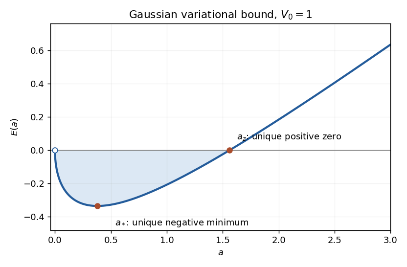
As $a\downarrow 0$, $E(a)=-V_0\sqrt{a}+O(a)$ approaches zero from below; as $a\to \infty$, it tends to infinity. The sketch and variational inequality therefore give a negative energy for every $V_0>0$. Since this decaying potential has essential spectrum beginning at zero, at least one bound state exists for every positive well depth.

For small $V_0$, the minimizer is $a_{\ast }=V_0^2-3V_0^4+O(V_0^6)$. Substitution gives $E(a_{\ast })=-V_0^2/2+V_0^4/2+O(V_0^6)$. Meanwhile the potential is strictly greater than $-V_0$ except at a single point and the kinetic energy is nonnegative, so a normalized bound-state expectation is strictly greater than $-V_0$. Thus

The unique maximum-$M$ product state isApply the total lowering operator $J_{-}=J_{1-}+J_{2-}$ and normalize to obtain that multiplet. At the next highest remaining $M$, choose a normalized vector orthogonal to all previously constructed multiplets and annihilated by $J_{+}$. It is the next highest-weight state; lower it in the same way. Iterating produces every allowed total angular momentum and the Clebsch-Gordan coefficients.

For equal constituent spins, a total-spin singlet has $M=0$, so only the product basis vectors with opposite magnetic quantum numbers can occur. Acting with $J_{+}$ on the expansion and examining the coefficient of $|j,m+1{⟩}_1|j,-m{⟩}_2$ givesThus ${\alpha }_{m+1}=-{\alpha }_m$. Normalization requires $(2j+1)|{\alpha }_m{|}^2=1$. Choosing a conventional overall phase givesThe exponent is an integer even for half-integral $j$. Projecting the specified extreme product state onto this unique singlet gives the measurement probability

A Poisson structure is a smooth antisymmetric matrix field ${\omega }^{ab}$ defining a bracketthat obeys the Jacobi identity. Bilinearity, antisymmetry and the product rule follow from this formula; Jacobi is the remaining condition. Applying Jacobi to the coordinate functions givesThese are also sufficient: expanding Jacobi for arbitrary functions cancels all second-derivative terms by antisymmetry, leaving these coefficients multiplying their first derivatives.

For ${\omega }^{ab}={ϵ}^{abc}{x}^c$, the nonconstant function $f={\sum }_a(x^a{)}^2$ is a Casimir function of a Poisson manifold, becauseby symmetry of $x^b{x}^c$. This is the usual three-dimensional Lie-Poisson bracket.

Since the matrix $M$ is symmetric, ${\partial }_{d}H={\sum }_b{M}^{db}{x}^b$. The Hamilton equations are ${\dot{x}}^a=\{x^a,H\}$, and henceOne valid choice of coefficients is $Q^{abc}={\sum }_d{ϵ}^{adc}{M}^{db}$. If symmetric coefficients in $b,c$ are preferred, the same equations useIn vector notation the evolution is $(Mx)\times x$, consistent with the bracket convention and with preservation of $|x{|}^2$.