
Past exam of the mathematics course of the University of Cambridge 2008 ia Paper 3 12C ii Created 2026-09-24 Updated 2026-09-24
Past exam of the mathematics course of the University of Cambridge 2008 ia Paper 3 12C i Created 2026-09-24 Updated 2026-09-24
Past exam of the mathematics course of the University of Cambridge 2008 ia Paper 3 11C b Created 2026-09-24 Updated 2026-09-24
Past exam of the mathematics course of the University of Cambridge 2008 ia Paper 3 11C a Created 2026-09-24 Updated 2026-09-24
Past exam of the mathematics course of the University of Cambridge 2008 ia Paper 3 10C iii Created 2026-09-24 Updated 2026-09-24
Past exam of the mathematics course of the University of Cambridge 2008 ia Paper 3 10C ii Created 2026-09-24 Updated 2026-09-24
Past exam of the mathematics course of the University of Cambridge 2008 ia Paper 3 10C i Created 2026-09-24 Updated 2026-10-14
Past exam of the mathematics course of the University of Cambridge 2008 ia Paper 2 9F Solution Created 2026-09-24 Updated 2026-10-14
Let be the offspring probability generating function, and let , for . Given , the next generation is a sum of independent offspring counts. Multiplication of their probability generating functions givesTaking conditional expectation and then averaging provesThus is the -fold composition of with itself. Induction makes this precise: it is true for , and composing once more gives the next generation. In particular , since both are the same iterated function. This is the generating-function recursion for a Galton-Watson process.
Write , initially assuming it is finite. The law of total expectation givesStarting at one therefore yields , with the value at understood to be one even if . Equivalently, differentiating the composition at one gives the same recurrence. If the offspring expectation is infinite, every positive generation has infinite expectation: a positive chance of at least one parent remains at each finite generation, and conditional on any positive parent count the next expected count is infinite.
For a Poisson branching process, . Extinction is absorbing because an empty generation has no parents, so extinction by generation is precisely . Hence . Using the composition in the order givesFor example is the chance of no offspring in the first generation. The recurrence includes the degenerate case , where extinction occurs in the first generation with certainty.
Past exam of the mathematics course of the University of Cambridge 2008 ia Paper 2 8A Solution Created 2026-09-24 Updated 2026-10-14
For this quartic potential with fourfold symmetry, the first derivatives factor:The critical points are the origin, the four axis points , and four points with both coordinates nonzero. At the latter, . Subtracting and using gives . Thus the complete list iswhere the two signs in the final group are chosen separately.
The Hessian isAt the origin it is , so there is a strict local minimum with value zero. At an axis point its eigenvalues are and , giving a saddle point of a scalar function if and a strict local maximum if . All four axis values are .
At a diagonal point the Hessian has eigenvaluesHence these four points are strict local maxima for and saddle points of a scalar function for . Their value is . None of these critical points is degenerate when .
To describe the level curves precisely, use polar coordinates and writeFor a level , the possible radii satisfyretaining only real, nonnegative values. This formula, together with reflection in each axis and interchange of the coordinates, determines the level curves. The radial maximum in a direction is , attained at . It also proves that the local maxima identified above are global: the largest directional value is on the diagonals if , and on the axes if .
For negative only the plus sign gives a positive radius, producing one outer closed level curve. At there is the isolated origin and the outer curve . For , where is the saddle value, both radial branches exist in every direction, giving an inner loop around the origin and an outer loop. At they meet at the four saddle points of a scalar function. Above the saddle value, four separate loops surround the four maxima; they shrink to those points at the maximum value. There are no level curves above it.
For , the saddle value is and the four high-level loops lie along the diagonals. For , and the four high-level loops lie along the coordinate axes. The sketches show representative values in both regimes; the highlighted level curve is the saddle level.
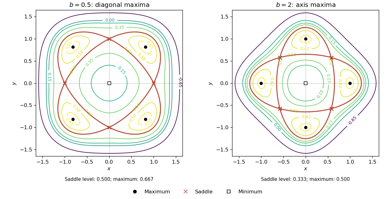
Contours of the fourfold quartic potential, with diagonal maxima for b less than one and axis maxima for b greater than one
. Details. 
Finally, at the expression depends only on radius:Consequently The maximum set is the whole unit circle, not merely four isolated points.
Past exam of the mathematics course of the University of Cambridge 2008 ia Paper 2 7A Solution Created 2026-09-24 Updated 2026-10-14
Write a power series . Substitution givesThe lowest coefficients give , , with free. For , matching the coefficient of gives the recurrenceAll odd coefficients consequently vanish. For the first solution, , , so the first three nonzero terms, when , areFor the second, , , givingIf its prescribed constant is zero, the corresponding solution is identically zero and has no nonzero terms.
For the change of variable, put , , with . The chain rule givesAfter division by , the coefficient of is and that of is . A genuine constant-coefficient equation requires , which both removes and makes the final coefficient constant. The transformed equation is .
This quadratic-variable reduction of a singular oscillator yieldsIt holds on each interval away from zero and both solutions extend smoothly through zero. Here and , so the specified solutions are exactly and . Their Taylor series agree with the recurrences above. Although the original equation has a regular singular point at zero, these two linearly independent smooth solutions supply the required data there.
Past exam of the mathematics course of the University of Cambridge 2008 ia Paper 2 6A Solution Created 2026-09-24 Updated 2026-10-14
With the indicated order of the two solutions, define the Wronskian byWhere , this gives the first-order linear differential equationIntegrating produces the reduction of order formulaThis formula is local on an interval where the known solution does not vanish; an arbitrary nonzero scaling of the linearly independent solution changes the normalization of .
Differentiate the Wronskian and use the differential equation for each solution:Thus , proving the Abel identity, and . For continuous coefficients on a nonsingular interval, linearly independent solutions have .
For the particular equation, write . The proposed solution is , with and , so substitution gives . Away from the singular point , division by gives . The Abel identity therefore giveswith a separate constant on each interval lying on one side of the singular point. The reduction of order integral is , soChoosing , givesThe nonzero Wronskian proves linear independence. Direct substitution also verifies the second solution, since . These solutions form a basis on either nonsingular interval; the second solution is not defined at .
Past exam of the mathematics course of the University of Cambridge 2008 ia Paper 2 5A v Created 2026-09-24 Updated 2026-09-24
Past exam of the mathematics course of the University of Cambridge 2008 ia Paper 2 5A iv Created 2026-09-24 Updated 2026-09-24
Past exam of the mathematics course of the University of Cambridge 2008 ia Paper 2 5A iii Created 2026-09-24 Updated 2026-09-24
Past exam of the mathematics course of the University of Cambridge 2008 ia Paper 2 5A ii Created 2026-09-24 Updated 2026-09-24
Past exam of the mathematics course of the University of Cambridge 2008 ia Paper 2 5A i Created 2026-09-24 Updated 2026-10-14
Past exam of the mathematics course of the University of Cambridge 2008 ia Paper 2 4F Solution Created 2026-09-24 Updated 2026-10-14
Let be one score. It has the discrete uniform distribution on , so its expected value and second moment areThereforeFor independent throws, linearity of expectation and additivity of variance give and . The sample average consequently has expectation and variance .
The Chebyshev inequality follows by applying the Markov inequality to the nonnegative square of a centered random variable. It givesThis is at most if . Thus suffices, as does every larger integer. This is the smallest integer guaranteed by this particular Chebyshev inequality bound; it need not be the smallest integer satisfying the actual probability requirement.
Past exam of the mathematics course of the University of Cambridge 2008 ia Paper 2 3F Solution Created 2026-09-24 Updated 2026-10-14
The sampling without replacement makes all unordered pairs equally likely. The count of red-red pairs is , while the count of mixed pairs is . Thus their probabilities satisfyand cancellation gives . Hence , with three black socks. The count of black-black pairs is also , soThe mixed, red-red and black-black probabilities are respectively , which add to one and verify the given ratio.
Past exam of the mathematics course of the University of Cambridge 2008 ia Paper 2 2A Solution Created 2026-09-24 Updated 2026-10-14
For the cubic population iteration, put . Its fixed points solveThus always exists. For there are alsowhenever the expression under the square root is positive, namely or . At these coincide with zero; at only zero exists.
The criterion for fixed point stability for an iteration is . To justify it, continuity of gives a small interval around the fixed point where . The mean value theorem then gives , so this interval is invariant and the error decreases geometrically. This proves local asymptotic stability rather than merely linear boundedness.
Here . At zero its value is , so zero is locally asymptotically stable for . At a nonzero fixed point it isThe strict inequality is equivalent to . Both nonzero real fixed points are therefore locally asymptotically stable on that interval. This proves the two requested existence ranges. The strict derivative criterion alone makes no conclusion at the endpoint multipliers of modulus one.
Past exam of the mathematics course of the University of Cambridge 2008 ia Paper 2 1A Solution Created 2026-09-24 Updated 2026-10-14
The complementary solution comes from the characteristic equation , whose roots are . It is thereforeFor the resonant exponential particular solution, the forcing is already a homogeneous exponential, so the method of undetermined coefficients needs the resonant trial . If , the identity when gives . Hence andThe decay condition first eliminates the growing exponential, . A nonzero combination of the sine and cosine has a fixed nonzero amplitude and cannot tend to zero, so as well. Both remaining exponential terms decay because . Finally , giving the unique answerThis is an instance of resonance in a differential equation: multiplication by supplies the particular solution when the forcing exponent is a simple characteristic root.
There are unlisted articles, also show them or only show them.