
Pressure upper bound for Hausdorff dimension 2026-10-14
Suppose shrinking interval covers of have length-power sums with logarithmic growth rate , and is strictly decreasing with zero . For every those sums tend to zero exponentially. The definition of Hausdorff measure then gives , hence the displayed upper bound. A matching lower bound requires additional information and does not follow from this covering argument alone.
Hausdorff dimension of the Cantor set 2026-10-14
The middle-third Cantor set has Hausdorff dimensionIts Lebesgue measure is zero, yet . These assertions measure different aspects of size: interval length is too coarse to distinguish this set from a null set, while the critical fractional measuring rule captures its remaining structure.
At level , the construction covers by intervals of diameter . Their total -cost isFor it tends to zero, proving the upper dimension bound. At it equals one, giving . For this particular cover's cost grows, but that alone would not prove a lower bound on Hausdorff measure.
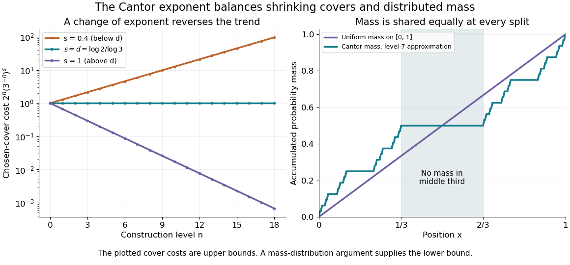
Cantor cover costs change trend at the critical exponent, and distributed mass supplies the lower bound
. Details. 
For the matching lower bound, use the Cantor distribution, which assigns mass to each level- Cantor cylinder. An interval of length with meets at most two level- construction intervals, since their gaps are at least . Its mass is therefore at mostEvery covering set of diameter in the line lies in an interval of length , so any small cover must have total -cost at least . This is the mass distribution principle in its interval form: , sufficient to prove the claimed dimension. The constants are convenient bounds, rather than an assertion of the exact critical Hausdorff measure. In the diagram, the right panel is a finite-stage approximation to the Cantor function, showing how probability is shared while the middle third receives none.
The reusable pattern is to obtain an upper bound by constructing covers and a lower bound by distributing mass. The same strategy underlies Cartesian powers of the Cantor set and the dimension formula for a finite similarity iterated function system satisfying the open set condition.
Mass distribution principle 2026-10-14
The mass distribution principle converts a diffuse measure into a lower bound on Hausdorff dimension. Let and let a Borel probability measure give a Borel set full mass. If, for some , every ball centered in satisfiesthen in the diameter-cost convention, and consequently .
The idea is to keep unit mass from being crowded into cheap covering pieces. For a piece of positive diameter meeting , choose . A ball of radius contains ; letting gives , where is the associated outer measure. Zero-diameter pieces have zero mass by the same estimate. For any sufficiently small cover,Thus every cover costs at least . This is the lower-bound counterpart to the explicit covers in scale-restricted Hausdorff content. The Cantor distribution supplies the needed mass in Hausdorff dimension of the Cantor set. [ref]
https://www.math.stonybrook.edu/~bishop/fractalbook.pdf. Bishop and Peres, §1.2: the mass distribution principle
.Uniform fixed-aspect rectangle crossing in bond percolation bounds at the self-dual parameter yield a positive lower bound for closed dual circuits in geometrically spaced disjoint annuli. The independent annular barriers for percolation imply that an origin-to-infinity open graph path has probability zero. Parameter monotonicity gives zero percolation probability for every .
For a positive harmonic function on the unit disc, choose a global harmonic conjugate and apply the Carathéodory derivative bound for the right half-plane to . This gives by the Cauchy-Riemann equations. A disk automorphism sending zero to has derivative modulus , so the chain rule gives the displayed bound. Composing a boundary-pole Poisson kernel with a disk automorphism attains equality, proving the coefficient is optimal at every point.
Brownian exit law from a quadrant 2026-10-14
Planar Brownian motion started at , , exits the positive quadrant through either positive coordinate axis with probability one-half. The density along each axis is for , measured with respect to distance along that axis. Squaring maps the quadrant to the upper half-plane and sends the starting point to . The boundary square therefore has the centered Cauchy distribution of scale ; pulling it back by gives the displayed density. The radius has distribution function , independently of which axis is chosen. There is no atom at the origin.
Hamming ball volume exponent 2026-10-14
For , the exponential growth rate of a q-ary Hamming ball is . Stirling's formula gives the exponent of each summand , and the sum lies between its largest term and times that term. Above the entropy-maximizing radius fraction, the exponent is one.
// Target: algebra.bigb
Icosian game 2026-10-14
The Icosian game made the vertex-visit puzzle tangible. The report of its 1857 presentation describes a plane projection of a regular dodecahedron, with holes at the vertices for ivory pins. The Trinity College Dublin archive connects this game with the search for closed routes visiting each vertex exactly once. This puzzle supplies a historical illustration of the Hamilton cycle requirement.[ref]
The Icosian Calculus, Hamilton papers archive. The Icosian Calculus, Hamilton papers archive: opening historical introduction and quoted report of the 1857 British Association presentation: dodecahedron projection and ivory pins
Weighted Hamilton cycle 2026-10-14
A weighted Hamilton cycle is a Hamilton cycle in a weighted graph, with cost equal to the sum of its traversed edge weights. Here weights represent symmetric nonnegative costs, rather than conductances. Asking whether a Hamilton cycle exists is a feasibility question; asking for the cheapest one is an instance of the travelling salesman problem. A complete graph supplies every possible connection between distinct vertices, making feasibility automatic for , while choosing the cheapest visiting order remains a separate mathematical optimization problem.
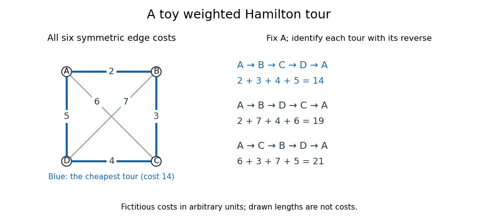
A fictitious weighted graph on four vertices: its three Hamilton cycles, identified under reversal and cyclic rotation, have costs 14, 19 and 21
. Details. 
Assign the complete graph the symmetric edge costs , , , , and , in arbitrary units. Fix the start at and identify each Hamilton cycle with its reverse. The three possibilities areThese exhaust the possibilities: the permutations of the other three vertices give orders, paired into three reversals. Hence the perimeter tour really is optimal for this toy instance. The diagram's geometric lengths are not costs, and no triangle inequality is assumed.
The usefulness of this model is to distinguish visiting required sites from covering required connections. If tasks are assigned to vertices and the route must return after one visit to each, a weighted Hamilton cycle captures the ordering requirement. If the job instead requires each edge once, the relevant object is an Euler circuit. The shortest path problem asks only for a cheapest route between specified endpoints. A 1954 primary research paper gave a concrete motivation for the travelling salesman problem: certify that a particular tour through 49 cities has minimum road-distance cost.[ref]
Solution of a Large-Scale Traveling-Salesman Problem by George B. Dantzig and others. Solution of a Large-Scale Traveling-Salesman Problem by G. Dantzig, R. Fulkerson and S. Johnson, abstract; Journal of the Operations Research Society of America 2(4), pp. 393–410 (1954)
These are abstract route models. If a cost stands for a whole graph path through an underlying network, travelling between consecutive task vertices can pass through intermediate network vertices more than once. One visit per task therefore does not imply one visit per physical junction. One-way connections require a directed graph; changing costs or extra timing constraints require a richer model than the fixed symmetric toy instance.
Necessary conditions for a Hamilton cycle 2026-10-14
A Hamiltonian graph must be a connected graph and have minimum degree : each vertex has two distinct neighbours on its Hamilton cycle. It also has no cut vertex. Indeed, deleting any vertex from the Hamilton cycle leaves a graph path through every remaining vertex, so the remaining graph is connected. These are quick ways to rule out a Hamilton cycle.[ref]
Hamilton Cycles. Diestel, Graph Theory, §10.1, printed pp. 323–324: necessary minimum degree two and 2-connectivity
Even these conditions together are not sufficient: the complete bipartite graph is connected, has minimum degree two and no cut vertex, but has no Hamilton cycle. Every graph cycle in a bipartite graph alternates between its two parts, using equally many vertices from each; it cannot use all two and all three.
In the other direction, Dirac's theorem gives a sufficient condition: a finite simple graph with and has a Hamilton cycle. Failure of this inequality proves nothing by itself: the cycle graph has a Hamilton cycle despite .[ref]
Hamiltonian graph 2026-10-14
A Hamiltonian graph is a graph containing a Hamilton cycle. This describes existence of a spanning graph cycle, rather than requiring every edge of the graph to belong to that graph cycle. In the finite simple graph convention, is a Hamiltonian graph for , because any ordering of its vertices closes using available edges.
Hall coefficient 2026-10-14
The Hall coefficient relates a transverse electric field to longitudinal current density and transverse magnetic field, with oriented axes as in the displayed formula. Its SI unit is . For one isotropic Drude model species it is ; multiple charge carriers need not follow that formula.
For a finite nonempty integer set , put . If an integer , some of size at least has a Freiman 2-isomorphism into . Choose an auxiliary prime so large that reduction is injective on and every nonzero element of remains nonzero. Dilate modulo by a uniformly chosen nonzero multiplier. The forbidden residues are those represented by nonzero multiples of of absolute value less than , at most residues. The nonzero elements of occur in opposite pairs; the two elements in each pair have the same bad event. The union bound therefore gives failure probability at most . Choose a multiplier avoiding all these events. Select the more populated of two half-intervals of residues modulo . Differences of two pair sums of representatives then have absolute value less than . An original additive relation must therefore lift to equality in the integers; conversely an equality modulo cannot have a nonzero lifted difference, by the forbidden-residue choice. Reduction modulo is the required isomorphism.
Weierstrass half-period translation formula 2026-10-14
Let represent a nonzero two-torsion point of a complex torus, and write . The product is an elliptic function whose apparent poles cancel against double zeros. It is therefore constant by Liouville theorem. Its value at is . The Weierstrass elliptic differential equation gives , proving the formula.
Let be the weights of the cubic Stokes dispersion symmetry and set . Orient with on its left. Evaluating the global relation at its two lower-half-plane roots and interpolating the linear expression removes both unknown boundary traces. The resulting Fokas method formula isThe discarded transform of the solution is holomorphic in and has zero integral after closing its contour for . Initial compatibility and sufficient smoothness and spatial decay are required. At the boundary, use a fixed time horizon later than before Fourier inversion, to avoid an endpoint half-value.
For with , the dispersion relation is and its symmetry is . On the upper domain , and therefore . After removing the unknown trace through the global relation, deform the boundary contour to the displayed two rays, with , oriented from left infinity to to right infinity. The factor decays like , while has Gaussian decay for large . Apparent poles introduced by splitting a finite-time forcing transform must be treated as removable singularities of the unsplit expression.
The baryon octet has rows with isospins , , . The central weight has two states, and . The baryon decuplet has rows with isospins . The three-quark flavour singlet has one state at the origin. Both abstract octet copies in share the same weights.
The Haar projection replaces a function by its mean on each dyadic interval of length . For a function satisfying Lipschitz continuity with constant , every value in a cell differs from its cell mean by at most . This bound holds for all points with a consistent endpoint convention, and requires no global L2 norm assumption when the projection is defined by local averages.
Pure growing-mode scaled velocity 2026-10-14
For a pure scalar growing density contrast with time-independent boundary conditions, fixes the scaled peculiar gravitational potential up to an irrelevant constant. The linearized continuity equation fixes the longitudinal scaled velocity to . The remaining homogeneous velocity is ; a divergence-free such field does not change the growing density at linear order. Excluding this decaying velocity component is necessary for time-independent . In an Einstein-de Sitter universe, and , furnishing a counterexample if the pure growing-velocity hypothesis is omitted.
Denominators in grouped birth-outcome models 2026-10-14
For each treatment year let be cycles, singleton deliveries, twin deliveries and deliveries of three or more babies. A singleton-per-cycle model uses . A multiple-delivery model conditional on a live delivery instead uses . The latter denominator counts deliveries, not babies, and it excludes failed cycles. Confusing these denominators changes the statistical question.
There are unlisted articles, also show them or only show them.